
House prices: what a missing value means, and when it matters
2,930 home sales with 82 columns, a right-skewed price, and missing values of three different kinds. Dropping incomplete rows loses most of the data and costs accuracy; between imputation strategies the difference is nil. Absence tracks price in the raw table, but through "no garage" and through neighbourhood, not on its own. How to classify missingness before treating it, and how to tell whether absence is a signal.
“Lots of missing values” is a symptom, not a diagnosis. In one table a blank means the field was not recorded; in another it means the thing does not exist; in a third it means the question did not apply. Each needs a different treatment, and the wrong one either throws away data or teaches the model something false. This study classifies the gaps in a well-known housing table, measures what each treatment costs, and checks whether absence itself predicts the price.
The data: residential sales in Ames, Iowa, 2006 to 2010 (ames_housing.tsv, De Cock, Journal of Statistics Education, 2011). One row per sale, 82 columns describing the lot, the building, its rooms, garage, basement and condition, and the sale price.
The question, as it arrived: “Predict the sale price.”
1. Understand the data
import pandas as pd, numpy as np

df = pd.read_csv("ames_housing.tsv", sep="\t")
df.columns = [c.replace(" ", "_").replace("/", "_") for c in df.columns]
print(df.shape, "| sold:", df["Yr_Sold"].value_counts().sort_index().to_dict())
print("SalePrice: median %.0f, mean %.0f, max %.0f, skew %.2f | log price skew %.2f" % (df["SalePrice"].median(), df["SalePrice"].mean(), df["SalePrice"].max(), df["SalePrice"].skew(), np.log(df["SalePrice"]).skew()))
big = df["Gr_Liv_Area"] > 4000
print("houses with over 4,000 sq ft of living area:", big.sum(), df.loc[big, ["Gr_Liv_Area", "SalePrice", "Sale_Condition"]].to_dict("records"))
df = df[~big].copy()
df["logp"] = np.log(df["SalePrice"])
na = df.isna().mean().sort_values(ascending=False)
print("columns with missing values: %d of %d" % ((na > 0).sum(), df.shape[1]))
print(na[na > 0].round(3).head(14).to_string())
(2930, 82) | sold: {2006: 625, 2007: 694, 2008: 622, 2009: 648, 2010: 341}
SalePrice: median 160000, mean 180796, max 755000, skew 1.74 | log price skew -0.01
houses with over 4,000 sq ft of living area: 5 [{'Gr_Liv_Area': 5642, 'SalePrice': 160000, 'Sale_Condition': 'Partial'}, {'Gr_Liv_Area': 4476, 'SalePrice': 745000, 'Sale_Condition': 'Abnorml'}, {'Gr_Liv_Area': 4316, 'SalePrice': 755000, 'Sale_Condition': 'Normal'}, {'Gr_Liv_Area': 5095, 'SalePrice': 183850, 'Sale_Condition': 'Partial'}, {'Gr_Liv_Area': 4676, 'SalePrice': 184750, 'Sale_Condition': 'Partial'}]
columns with missing values: 27 of 83
Pool_QC 0.996
Misc_Feature 0.964
Alley 0.932
Fence 0.805
Mas_Vnr_Type 0.606
Fireplace_Qu 0.486
Lot_Frontage 0.168
Garage_Cond 0.054
Garage_Yr_Blt 0.054
Garage_Finish 0.054
Garage_Qual 0.054
Garage_Type 0.054
Bsmt_Exposure 0.028
BsmtFin_Type_2 0.028One row is one sale. The price is right-skewed (mean well above median, skew 1.7) and its log is symmetric, so the models below fit log price; see regression on a skewed target. Five houses have over 4,000 square feet of living area, three of them sold at oddly low prices as partial sales; the dataset’s author documents them as unrepresentative and recommends removing them, which is done here and stated. Twenty-seven columns have gaps, from 0.03% to 99.6%.
2. Three kinds of missing
The columns with the most gaps are the ones about things a house may not have.
pairs = [("Garage_Type", "Garage_Area"), ("Bsmt_Qual", "Total_Bsmt_SF"), ("Fireplace_Qu", "Fireplaces"), ("Mas_Vnr_Type", "Mas_Vnr_Area")]
for quality, size in pairs:
    missing = df[quality].isna()
    print("%-13s missing in %4d rows; of those, %-13s == 0 in %4d" % (quality, missing.sum(), size, (missing & (df[size].fillna(0) == 0)).sum()))
print("Lot_Frontage missing: %d rows (%.1f%%) | share missing by lot configuration:" % (df["Lot_Frontage"].isna().sum(), 100 * df["Lot_Frontage"].isna().mean()),
      df.groupby("Lot_Config")["Lot_Frontage"].apply(lambda s: s.isna().mean()).round(2).to_dict())
Garage_Type missing in 157 rows; of those, Garage_Area == 0 in 157
Bsmt_Qual missing in 80 rows; of those, Total_Bsmt_SF == 0 in 80
Fireplace_Qu missing in 1422 rows; of those, Fireplaces == 0 in 1422
Mas_Vnr_Type missing in 1774 rows; of those, Mas_Vnr_Area == 0 in 1767
Lot_Frontage missing: 490 rows (16.8%) | share missing by lot configuration: {'Corner': 0.2, 'CulDSac': 0.49, 'FR2': 0.24, 'FR3': 0.29, 'Inside': 0.13}- Structural. Garage quality is missing in exactly the rows where garage area is zero; the same for basement, fireplace and masonry veneer. The blank means there is no garage. The right value is a category of its own (“None”) and a zero for the associated sizes, and a model that drops these rows would be dropping every house without a garage.
- Not applicable. Pool quality (99.6% missing), fence, alley: the same kind, at the extreme.
- Not recorded. Lot frontage is missing in 17% of rows, and the share depends on the lot’s shape: half of cul-de-sac lots have no frontage recorded, presumably because the measurement is ambiguous there. This is the only column where “missing” plausibly means “unknown”, and its missingness is related to other columns, which is what decides whether imputation can be simple.
3. Does absence track the price?
def price_gap(col):
    m = df[col].isna()
    return np.exp(df.loc[m, "logp"].mean() - df.loc[~m, "logp"].mean()) - 1

for col in ("Garage_Type", "Bsmt_Qual", "Fireplace_Qu", "Lot_Frontage"):
    print("%-13s typical price when missing, relative to present: %+.0f%%" % (col, 100 * price_gap(col)))
m = df["Lot_Frontage"].isna()
within = df.groupby("Neighborhood")[["Lot_Frontage", "logp"]].apply(lambda g: g.loc[g["Lot_Frontage"].isna(), "logp"].mean() - g.loc[g["Lot_Frontage"].notna(), "logp"].mean()).dropna()
print("Lot_Frontage: log-price gap (missing minus present) overall %+.3f | averaged within %d neighbourhoods %+.3f" % (df.loc[m, "logp"].mean() - df.loc[~m, "logp"].mean(), len(within), within.mean()))
Garage_Type typical price when missing, relative to present: -42%
Bsmt_Qual typical price when missing, relative to present: -41%
Fireplace_Qu typical price when missing, relative to present: -34%
Lot_Frontage typical price when missing, relative to present: +7%
Lot_Frontage: log-price gap (missing minus present) overall +0.066 | averaged within 24 neighbourhoods +0.003Houses with no garage sell for about 40% less, with no basement about 40% less, with no fireplace about a third less. That is real and it is not about missingness; it is about garages. A garage indicator would carry it, but so does garage area, which is zero for the same rows.
Lot frontage is the interesting one. Overall, houses with the frontage missing sell for 7% more. Within a neighbourhood the gap is essentially zero. The missingness is informative in the raw table only because cul-de-sac lots cluster in newer, pricier neighbourhoods. A missing-value indicator for this column would be a weak proxy for neighbourhood, which the model already has. This is the check to run before claiming “missingness predicts the target”: condition on the obvious confounder and see whether the association survives. See Simpson’s paradox and grouped confounding for the general pattern.
4. What each treatment costs
Chronological by year of sale: 2006 to 2008 train, 2009 and 2010 test. Nineteen numeric and twelve categorical columns, chosen for coverage rather than tuned. Five treatments of the gaps, one ridge regression on log price, with every imputation value learned on the training rows.
from sklearn.linear_model import Ridge

num = ["Lot_Frontage", "Lot_Area", "Overall_Qual", "Overall_Cond", "Year_Built", "Year_Remod_Add", "Mas_Vnr_Area", "Total_Bsmt_SF", "Gr_Liv_Area",
       "Full_Bath", "Half_Bath", "Bedroom_AbvGr", "TotRms_AbvGrd", "Fireplaces", "Garage_Cars", "Garage_Area", "Garage_Yr_Blt", "Wood_Deck_SF", "Open_Porch_SF"]
cat = ["Neighborhood", "MS_Zoning", "Bldg_Type", "House_Style", "Exter_Qual", "Kitchen_Qual", "Bsmt_Qual", "Garage_Type", "Garage_Finish", "Fireplace_Qu", "Central_Air", "Sale_Condition"]
tr, te = df[df["Yr_Sold"] <= 2008], df[df["Yr_Sold"] >= 2009]
print("train: sold 2006-2008, %d houses | test: sold 2009-2010, %d houses | rows with a gap in at least one used column: %.1f%%" % (len(tr), len(te), 100 * df[num + cat].isna().any(axis=1).mean()))
fill = {"median": tr[num].median(), "frontage_by_nbhd": tr.groupby("Neighborhood")["Lot_Frontage"].median()}      # learned on training rows only

def prepare(frame, strategy, columns=None):
    X, C = frame[num].copy(), frame[cat].copy()
    if strategy == "indicators":
        for c in ("Lot_Frontage", "Garage_Yr_Blt", "Mas_Vnr_Area"):
            X[c + "_missing"] = X[c].isna().astype(float)
    if strategy == "structural":
        for c in ("Mas_Vnr_Area", "Total_Bsmt_SF", "Garage_Cars", "Garage_Area"):
            X[c] = X[c].fillna(0.0)
        X["Garage_Yr_Blt"] = X["Garage_Yr_Blt"].fillna(X["Year_Built"])
        C = C.fillna("None")
    if strategy == "neighbourhood":
        X["Lot_Frontage"] = X["Lot_Frontage"].fillna(frame["Neighborhood"].map(fill["frontage_by_nbhd"]))
    X = X.fillna(fill["median"])
    C = C.fillna("Missing")
    D = pd.concat([X, pd.get_dummies(C.astype(str), dtype=float)], axis=1)
    return D if columns is None else D.reindex(columns=columns, fill_value=0.0)

def rmse(y, yhat):
    return np.sqrt(np.mean((y - yhat) ** 2))

results = {}
def run(strategy, label):
    a, b = (tr.dropna(subset=num + cat), te.dropna(subset=num + cat)) if strategy == "drop rows" else (tr, te)
    Xa = prepare(a, strategy)
    Xb = prepare(b, strategy, Xa.columns).fillna(fill["median"])
    mu, sd = Xa.mean(), Xa.std().replace(0, 1)
    p = Ridge(alpha=3.0).fit(((Xa - mu) / sd).values, a["logp"].values).predict(((Xb - mu) / sd).values)
    results[label] = rmse(b["logp"].values, p)
    print("%-46s train %4d  test %4d | RMSE of log price %.4f | median abs error $%5.0f" % (label, len(a), len(b), results[label], np.median(np.abs(np.exp(b["logp"].values) - np.exp(p)))))

run("drop rows", "drop every row with a gap")
run("median", "median, and 'Missing' as a category")
run("indicators", "median + missing indicators")
run("structural", "structural: 0 and 'None' where absence means none")
run("neighbourhood", "Lot_Frontage from the neighbourhood median")
train: sold 2006-2008, 1936 houses | test: sold 2009-2010, 989 houses | rows with a gap in at least one used column: 60.5%
drop every row with a gap train 768 test 386 | RMSE of log price 0.1502 | median abs error $12547
median, and 'Missing' as a category train 1936 test 989 | RMSE of log price 0.1319 | median abs error $10197
median + missing indicators train 1936 test 989 | RMSE of log price 0.1319 | median abs error $10277
structural: 0 and 'None' where absence means none train 1936 test 989 | RMSE of log price 0.1319 | median abs error $10140
Lot_Frontage from the neighbourhood median train 1936 test 989 | RMSE of log price 0.1320 | median abs error $10347Dropping incomplete rows discards more than half the training data (a house with no fireplace has a gap in the fireplace quality column) and the error rises by about 14%. Every other treatment gives the same number to three decimals. The indicators are harmless and useless, because the information they carry is already in the table: “no garage” is in garage area, “cul-de-sac” is in the neighbourhood dummies. The structural encoding is the correct one, and it is correct without being better, which is what a well-designed table looks like: the zero sizes carry the absence.
5. Would the treatment ever matter here?
If the encoding of a blank is going to matter, it will be when the blank is the only record of the fact. Take the garage sizes away, so that the only garage information is the quality columns whose blanks mean “none”, and see how much the “None” level recovers.
num_no_garage = [c for c in num if not c.startswith("Garage")]

def garage_variant(keep_quality, label):
    cols_c = cat if keep_quality else [c for c in cat if not c.startswith("Garage")]
    def prep(frame, columns=None):
        D = pd.concat([frame[num_no_garage].fillna(fill["median"]), pd.get_dummies(frame[cols_c].fillna("None").astype(str), dtype=float)], axis=1)
        return D if columns is None else D.reindex(columns=columns, fill_value=0.0)
    Xa = prep(tr)
    Xb = prep(te, Xa.columns)
    mu, sd = Xa.mean(), Xa.std().replace(0, 1)
    p = Ridge(alpha=3.0).fit(((Xa - mu) / sd).values, tr["logp"].values).predict(((Xb - mu) / sd).values)
    results[label] = rmse(te["logp"].values, p)
    print("%-62s RMSE of log price %.4f" % (label, results[label]))

garage_variant(False, "no garage columns at all")
garage_variant(True, "garage quality columns only, blank kept as its own level 'None'")
no garage columns at all RMSE of log price 0.1334
garage quality columns only, blank kept as its own level 'None' RMSE of log price 0.1331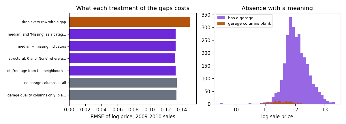
Show the code for this figure
import matplotlib.pyplot as plt

fig, (a1, a2) = plt.subplots(1, 2, figsize=(10, 3.6))
labels = list(results.keys())
a1.barh(range(len(labels)), [results[k] for k in labels], color=["#b45309"] + ["#6d28d9"] * 4 + ["#6b7280"] * 2)
a1.set_yticks(range(len(labels)))
a1.set_yticklabels([l if len(l) < 34 else l[:32] + "..." for l in labels], fontsize=7)
a1.invert_yaxis()
a1.set_xlabel("RMSE of log price, 2009-2010 sales")
a1.set_title("What each treatment of the gaps costs")
has = df["Garage_Type"].notna()
a2.hist(df.loc[has, "logp"], bins=40, alpha=0.7, color="#6d28d9", label="has a garage")
a2.hist(df.loc[~has, "logp"], bins=40, alpha=0.9, color="#b45309", label="garage columns blank")
a2.set_xlabel("log sale price")
a2.set_title("Absence with a meaning")
a2.legend(fontsize=8)
fig.tight_layout()
fig.savefig("ames-missing-treatments.png", dpi=120)
plt.show()
Almost nothing. Removing every garage column costs 0.0015 in RMSE, and keeping the quality columns with the blank as “None” recovers a fifth of that. The reason is the same as before: this table is redundant. Overall quality, year built and neighbourhood already say most of what “no garage” says about the price. The honest conclusion is that on this table the treatment of missing values cannot matter much, however it is done, because absence is recorded three times over. That is a property of a well-designed table, not of missing values in general; on a thin table where the blank is the only record of the fact, the same experiment will come out differently, and it is worth running to find out which kind of table you have.
6. What to say
Twenty-seven of the 82 columns have gaps, but nearly all of them are structural: the blank in “garage quality” is the 157 houses without a garage, and so on for basements, fireplaces and pools. Treated that way, as a category of their own with zero sizes, they cost nothing. The one genuinely unrecorded column, lot frontage, is missing mostly on cul-de-sac lots, and its apparent association with higher prices disappears within neighbourhoods. On a chronological split a ridge regression on log price reaches an RMSE of 0.132 in log units, about a 13% typical error, under any sensible imputation; dropping incomplete rows loses most of the data and raises the error to 0.150. The only way to lose accuracy to missingness here is to delete it.
Takeaways
- Classify every gap before treating it: structural (the thing does not exist), not applicable, or not recorded. The check is whether the blank lines up with a zero size or a related column.
- Absence with a meaning is a value. Encode it as its own level and zero sizes. Do not drop the column for being “mostly missing” and do not drop the rows.
- Before claiming missingness predicts the target, condition on the obvious confounder. Lot-frontage gaps looked informative and were a proxy for neighbourhood.
- Missing indicators are cheap insurance, harmless when redundant, and the only thing that can help when the absence is the only record of the fact. Test which case you are in by removing the correlated columns; here nothing came back, because nothing was lost.
- Dropping rows is the expensive option, and it also changes what population the model describes.
- Learn every imputation value on the training rows. A test-period median is a small leak; a test-period neighbourhood median is a larger one.
Related: the bank marketing table, where “unknown” is a category and −1 is a sentinel; leaked columns and labels that aren’t labels, where a zero meant “not recorded”; missing values for the reference version of this page.