
Evaluating predictive signals
Three questions turn "does this predict that?" into one number with an error bar. What picture would I see, how do I get many independent looks at it, and how do I summarise them. The result is the daily cross-sectional rank IC.
“Does yesterday’s X tell you anything about tomorrow’s Y?” is not yet a question a number can answer. Three further questions make it one, and the same three work for almost any signal on almost any panel.
Picture, repeats, summary
Picture. If the signal worked, what plot would I see? A scatter of signal against outcome, tilted. Correlation is the number for “how tilted”. Use rank correlation (Spearman) rather than Pearson, because financial quantities have fat tails and one extreme stock must not be allowed to decide the number. See Pearson vs Spearman.
Repeats. How do I get many independent looks at that picture? On a panel of many stocks over many days: one correlation per day, across the ~500 stocks that day. That gives ~1,250 numbers over five years. On a single series there is no cross-section, and the repeats have to be non-overlapping windows or years instead; see single series or panel.
Summary. The mean of those numbers is the headline. The t-statistic (mean over its standard error across days) says whether the mean is distinguishable from zero. The hit rate (share of days with a positive correlation) says whether it is consistent rather than carried by a few days.
That object is the daily cross-sectional rank information coefficient, or rank IC. The code is the same for every signal; only the column names change.
The code
import pandas as pd, numpy as np

df = pd.read_csv("all_stocks_5yr.csv")
df["date"] = pd.to_datetime(df["date"])
df = df.rename(columns={"Name": "ticker"}).sort_values(["ticker", "date"]).reset_index(drop=True)
per = df.groupby("ticker").size()
df = df[df["ticker"].isin(per[per >= 1000].index)].copy()
g = df.groupby("ticker")
df["ret"] = g["close"].pct_change()
df["fwd_ret"] = g["ret"].shift(-1)
df["sig1"] = -df["ret"]                       # the signal under test: short-term reversal
df = df.dropna(subset=["ret", "fwd_ret"])

cut, embargo = pd.Timestamp("2016-06-30"), pd.Timedelta(days=7)
train = df[df["date"] <= cut].copy()
test = df[df["date"] > cut + embargo].copy()

def daily_ic(d, sig, tgt="fwd_ret", method="spearman"):
    """One correlation per date between the signal and the target, across the cross-section."""
    return (d.groupby("date")[[sig, tgt]]
             .apply(lambda x: x[sig].corr(x[tgt], method=method))
             .dropna())

def report(ic, label):
    m, s, n = ic.mean(), ic.std(), len(ic)
    print("%-28s mean IC %+.4f   t = %+.2f   hit = %.2f   days = %d" % (label, m, m / (s / np.sqrt(n)), (ic > 0).mean(), n))

report(daily_ic(train, "sig1"), "reversal, train")
report(daily_ic(test, "sig1"), "reversal, test")
reversal, train mean IC +0.0114 t = +2.18 hit = 0.53 days = 854
reversal, test mean IC +0.0156 t = +1.98 hit = 0.55 days = 399groupby("date") gives the repeats. Selecting the two columns before apply keeps the code working across pandas versions (see portable pandas idioms). The report line is the whole summary: mean, t, hit rate, count.
Reading the number
An IC of 0.015 is tiny as a correlation. That is normal for a one-day-ahead return signal on liquid stocks; anything above 0.05 at that horizon deserves suspicion before celebration. What makes 0.015 worth reporting is the t-statistic and the hit rate: it is small and consistent, not large and lucky. Say it that way.
The t-statistic here treats each day’s IC as an independent draw. That is reasonable for one-day-ahead targets, and wrong for overlapping multi-day targets; see t-statistics from repeated looks.
Flip a coin 10,000 times and get 5,100 heads. The average is 0.01 above fair. One flip has standard deviation 0.5, and averaging 10,000 flips shrinks that by √10,000 = 100, to 0.005: the standard error. 0.01 / 0.005 = 2, and that is the t-stat. For a fair coin, landing 2 or more standard errors away happens about 5% of the time. So t ≈ 2 is borderline, and 4 or more is hard to call luck. Here each period’s IC plays the part of one flip.
This assumes the periods are independent. Overlapping targets (a 5-day return scored every day) make neighbouring ICs move together and inflate t.
Score the baseline beside the signal
The score above has nothing next to it. Two things fix that: a baseline scored the same way, and a lag that can’t reach across a gap. The block starts again from the full file, with the bad prints from the triage checks removed. The target here is the open-to-close return.
df = pd.read_csv("all_stocks_5yr.csv").rename(columns={"Name": "ticker"})
df["date"] = pd.to_datetime(df["date"])
df = df.sort_values(["ticker", "date"]).reset_index(drop=True)
df = df[~((df["close"] > df["high"]) | (df["close"] < df["low"]) | (df["high"] < df["low"]))].copy()   # bad prints out

df["ret"] = df["close"] / df["open"] - 1                              # target: open to close
gap = df.groupby("ticker")["date"].diff()
df["prev_ret"] = df.groupby("ticker")["ret"].shift(1)                 # baseline: last bar's return
df["sig"] = df["open"] / df.groupby("ticker")["close"].shift(1) - 1   # signal known at the open
lag_bad = gap > pd.Timedelta(days=4)            # daily equities: allow weekends; continuous data: gap != gap.median()
df.loc[lag_bad, ["prev_ret", "sig"]] = np.nan
print("lags blanked:", lag_bad.sum())

def ic(d, s, t="ret"):
    x = d.groupby("date")[[s, t]].apply(lambda z: z[s].corr(z[t], method="spearman")).dropna()
    return pd.Series({"IC": x.mean(), "t": x.mean() / (x.std() / np.sqrt(len(x))), "hit": (x > 0).mean(), "n": len(x)})

build = df[df["date"] < "2016-07-01"]
print(pd.DataFrame({s: ic(build, s) for s in ["sig", "prev_ret"]}).T.round(4))
lags blanked: 7
IC t hit n
sig -0.0564 -11.9030 0.3080 854.0
prev_ret 0.0112 2.4591 0.5398 854.0Over the build period (854 days), sig scores an IC of −0.0564 with t −11.90, and prev_ret scores +0.0112 with t +2.46. Seven lags were blanked across gaps longer than four days. The sign gives the direction: stocks that open further above yesterday’s close tend to do worse than the rest from open to close. Compare the sizes of the two ICs, not their signs.
- A lag must not reach across a gap. After an outage, a halt or a late listing,
shift(1)hands you a bar from hours or days earlier. Blank it. For continuous data (hourly, 24/7) the rule is exact:gap != gap.median(). For daily equities, allow weekends and long weekends. - Always put the baseline in the same table. If the simple baseline scores higher than your signal, that is a finding, and it goes on the slide. The next question is whether the signal adds anything beyond it: see does a signal add anything beyond a known baseline?
The picture itself: a binned scatter
A scatter of 200,000 points is unreadable. Bin the signal into deciles within each date and plot the mean outcome per decile. If the signal works the bars tilt; if it works monotonically, they tilt in order.
q = test.groupby("date")["sig1"].transform(lambda x: pd.qcut(x.rank(method="first"), 10, labels=False))
decile_means = test.groupby(q)["fwd_ret"].mean() * 1e4          # basis points per day
print(decile_means.round(2).tolist())
print("top minus bottom: %.2f bps/day" % (decile_means.iloc[-1] - decile_means.iloc[0]))
[2.56, 4.66, 5.2, 4.42, 5.96, 6.96, 5.79, 7.35, 5.54, 6.68]
top minus bottom: 4.12 bps/day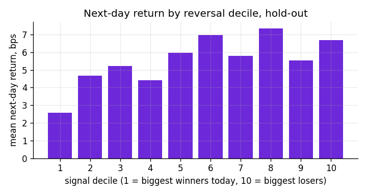
Tilted, not monotonic: the extreme deciles differ by about 4 basis points a day and the middle is noise. That is what an IC of 0.015 looks like. rank(method="first") breaks ties so that qcut always produces ten bins even when many signal values are equal.
Pearson and Spearman side by side
When the tails are fat the two disagree, and the disagreement is informative.
report(daily_ic(test, "sig1", method="pearson"), "reversal, test, Pearson")
report(daily_ic(test, "sig1", method="spearman"), "reversal, test, Spearman")
reversal, test, Pearson mean IC +0.0063 t = +0.81 hit = 0.53 days = 399
reversal, test, Spearman mean IC +0.0156 t = +1.98 hit = 0.55 days = 399Same data, same days. The Pearson version is dragged around by the handful of 25%+ moves and loses the effect; the rank version sees it. When a reader asks “why ranks?”, this pair of lines is the answer.
Other targets, same shape
- A binary outcome (up or down, big move or not): the picture is a hit rate against the majority-class rate, the repeats are still days, the summary is still a mean and a t. See logistic regression with a majority-class baseline.
- A size outcome (how large tomorrow’s move is): exactly the same code, different target column. The relative volume case study reaches an IC of 0.10, seven times the reversal IC, because sizes are far more predictable than signs.
- A single series (does the market’s return today predict tomorrow’s): no cross-section, so the repeats are years or quarters. See the market-level case study.
After the score
A score is not a result until it has been attacked: is it stable across the hold-out, does it survive removing the extreme rows, and could anyone use it after costs. And before it is a score, the protocol that defined it should have been frozen.