Charts as PNGs for slides

A slide gets one chart, the chart gets one message, and the whole thing is produced with matplotlib alone: no seaborn, no styling library, nothing that might not be installed. Every recipe ends the same way: save the PNG at 120 dpi for the slide, then plt.show() so the figure also appears in the notebook.

Setup once

In a notebook, never set the backend: matplotlib.use("Agg") is for scripts that only write files, and in Jupyter it stops every figure from displaying.

import pandas as pd, numpy as np
import matplotlib.pyplot as plt          # NOT matplotlib.use("Agg"): that line kills display in Jupyter

df = pd.read_csv("all_stocks_5yr.csv")
df["date"] = pd.to_datetime(df["date"])
df = df.rename(columns={"Name": "ticker"}).sort_values(["ticker", "date"]).reset_index(drop=True)
per = df.groupby("ticker").size()
df = df[df["ticker"].isin(per[per >= 1000].index)].copy()
g = df.groupby("ticker")
df["ret"] = g["close"].pct_change()
df["fwd_ret"] = g["ret"].shift(-1)
df["signal"] = -df["ret"]                # <- the SIGNAL column goes on the x-axis / into the IC, never the baseline
df = df.dropna(subset=["ret", "fwd_ret"])
cut, embargo = pd.Timestamp("2016-06-30"), pd.Timedelta(days=7)
test = df[df["date"] > cut + embargo].copy()

def daily_ic(d, sig, tgt="fwd_ret"):
    return d.groupby("date")[[sig, tgt]].apply(lambda x: x[sig].corr(x[tgt], method="spearman")).dropna()

train = df[df["date"] <= cut]

A figure of 8 by 3.2 inches at 120 dpi is 960 by 384 pixels: wide and short, which leaves room on a slide for a title and one sentence. Use 6 by 3.2 for a chart that sits beside text.

1. Cumulative IC over the hold-out

Use it when: asked “how does it look over time?” A line that climbs steadily is a consistent signal; one that climbs and then flattens is a signal that stopped.

# ---- Figure 1: cumulative daily IC line (slide 6) ----
ic = daily_ic(test, "signal")
fig, ax = plt.subplots(figsize=(8, 3.2))
ic.cumsum().plot(ax=ax)
ax.axhline(0, color="k", lw=0.8)
ax.set_title("Cumulative daily rank IC, hold-out  (mean %+.4f, t %+.2f, %d days)" % (ic.mean(), ic.mean() / (ic.std() / np.sqrt(len(ic))), len(ic)))
ax.set_ylabel("cumulative IC"); ax.set_xlabel("")
fig.tight_layout()
fig.savefig("fig_cum_ic.png", dpi=120)    # 1. save first, for PowerPoint
plt.show()                                # 2. then show, so it appears in the notebook
                                          # 3. no plt.close() here; only inside loops that make many figures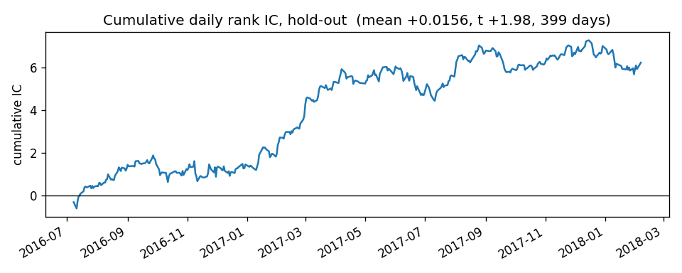

2. Mean outcome by signal decile

Use it when: asked “is it monotone?” The picture behind an IC: bars that tilt.

# ---- Figure 2: decile bar chart (slide 4 or 6) ----
test["dec"] = test.groupby("date")["signal"].transform(lambda x: pd.qcut(x.rank(method="first"), 10, labels=False))
dec = test.groupby("dec")["fwd_ret"].mean() * 1e4
fig, ax = plt.subplots(figsize=(6, 3.2))
ax.bar(dec.index + 1, dec.values)
ax.axhline(0, color="k", lw=0.8)
ax.set_xlabel("signal decile (1 = lowest, 10 = highest)"); ax.set_ylabel("mean next-day return, bps")
ax.set_title("Mean target by signal decile, hold-out")
fig.tight_layout()
fig.savefig("fig_deciles.png", dpi=120)
plt.show()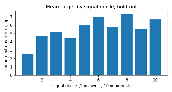

3. Rolling 60-day IC

Use it when: asked “is it stable?”

ic_tr, ic_te = daily_ic(train, "signal"), daily_ic(test, "signal")

# ---- Figure 3: rolling 60-day IC. Use it when: asked "is it stable?" ----
fig, ax = plt.subplots(figsize=(8, 3.2))
ic_te.rolling(60).mean().plot(ax=ax)
ax.axhline(0, color="k", lw=0.8)
ax.axhline(ic_te.mean(), color="grey", ls="--", lw=0.8)
ax.set_title("Rolling 60-day mean IC, hold-out (dashed = full-period mean)")
ax.set_ylabel("IC"); ax.set_xlabel("")
fig.tight_layout()
fig.savefig("fig_rolling_ic.png", dpi=120)
plt.show()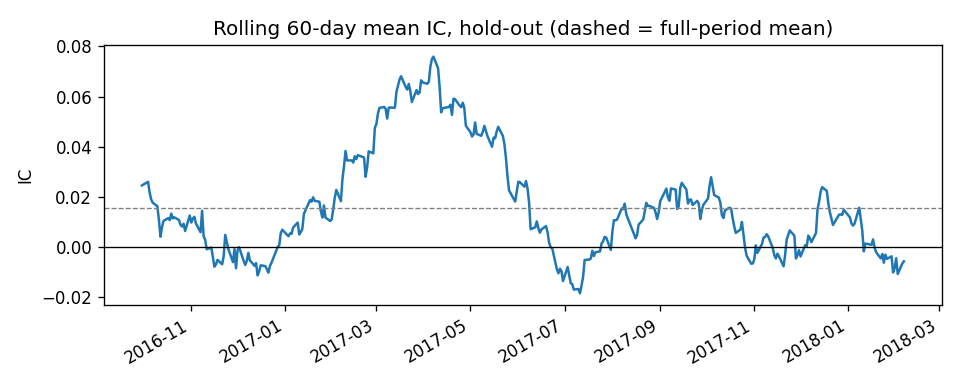

4. Build against hold-out, with error bars

Use it when: asked “does it survive out of sample?”

# ---- Figure 4: build vs hold-out with error bars. Use it when: asked "does it survive out of sample?" ----
se = lambda s: s.std() / np.sqrt(len(s))
means = [ic_tr.mean(), ic_te.mean()]; errs = [2 * se(ic_tr), 2 * se(ic_te)]
fig, ax = plt.subplots(figsize=(4, 3.2))
ax.bar(["build", "hold-out"], means, yerr=errs, capsize=6)
ax.axhline(0, color="k", lw=0.8)
ax.set_ylabel("mean daily IC (bars = ±2 s.e.)")
ax.set_title("Same signal, before and after the cut")
fig.tight_layout()
fig.savefig("fig_build_vs_holdout.png", dpi=120)
plt.show()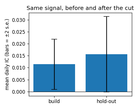

5. The input’s distribution, tails clipped

Use it when: slide 2, “what does the input look like?”

# ---- Figure 5: signal distribution, tails clipped. Use it when: slide 2, "what does the input look like?" ----
lo, hi = df["signal"].quantile([0.005, 0.995])
fig, ax = plt.subplots(figsize=(6, 3.2))
df["signal"].clip(lo, hi).plot.hist(bins=80, ax=ax)
ax.set_title("Signal distribution, clipped at 0.5% / 99.5%")
ax.set_xlabel("signal"); ax.set_ylabel("rows")
fig.tight_layout()
fig.savefig("fig_signal_hist.png", dpi=120)
plt.show()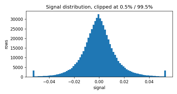

6. Top-minus-bottom decile in bps

Use it when: asked “is it big?” An IC has no units; costs are in bps.

# ---- Figure 6: top-minus-bottom decile in bps. Use it when: asked "is it big?" (an IC has no units; costs are in bps) ----
test["dec"] = test.groupby("date")["signal"].transform(lambda x: pd.qcut(x.rank(method="first"), 10, labels=False))
top = test[test["dec"] == 9].groupby("date")["fwd_ret"].mean()
bot = test[test["dec"] == 0].groupby("date")["fwd_ret"].mean()
spread = (top - bot) * 1e4
fig, ax = plt.subplots(figsize=(8, 3.2))
spread.cumsum().plot(ax=ax)
ax.axhline(0, color="k", lw=0.8)
ax.set_title("Cumulative top-minus-bottom decile, bps (mean %.1f bps/day, before costs)" % spread.mean())
ax.set_ylabel("cumulative bps"); ax.set_xlabel("")
fig.tight_layout()
fig.savefig("fig_spread_bps.png", dpi=120)
plt.show()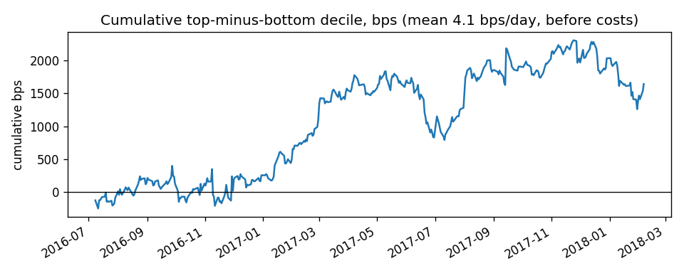

7. Net return against transaction cost

Use it when: asked “could anyone trade it?” A straight line crossing zero at the break-even cost.

def long_short(d, sig):
    def one(x):
        q = pd.qcut(x[sig].rank(method="first"), 10, labels=False)
        return x.loc[q == 9, "fwd_ret"].mean() - x.loc[q == 0, "fwd_ret"].mean()
    return d.groupby("date")[[sig, "fwd_ret"]].apply(one).dropna()

def turnover(d, sig):
    tops = d.groupby("date")[[sig, "ticker"]].apply(lambda x: set(x.loc[pd.qcut(x[sig].rank(method="first"), 10, labels=False) == 9, "ticker"]))
    return float(np.mean([1 - len(a & b) / max(len(a), 1) for a, b in zip(tops.values[:-1], tops.values[1:])]))

gross = long_short(test, "signal").mean() * 1e4
to = turnover(test, "signal")
costs = np.arange(0, 12.1, 0.5)
net = gross - 2 * to * costs
be = gross / (2 * to)

fig, ax = plt.subplots(figsize=(6, 3.2))
ax.plot(costs, net); ax.axhline(0, color="k", lw=0.8); ax.axvline(be, color="r", ls="--", lw=0.8)
ax.set_xlabel("round-trip cost, bps"); ax.set_ylabel("net bps / day")
ax.set_title("Net return vs transaction cost: break-even at %.1f bps" % be)
fig.tight_layout()
fig.savefig("fig_cost_sweep.png", dpi=120)
plt.show()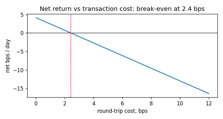

8. Histogram of the target with its tails

Use it when: the data-quality slide. A log-scale y axis is what makes the tails visible.

fig, ax = plt.subplots(figsize=(8, 3.2))
ax.hist(df["ret"], bins=400, range=(-0.3, 0.3))
ax.set_yscale("log")
ax.set_xlabel("daily return"); ax.set_ylabel("rows (log scale)")
ax.set_title("Daily returns: the tails go far past what a normal distribution allows")
fig.tight_layout()
fig.savefig("fig_hist.png", dpi=120)
plt.show()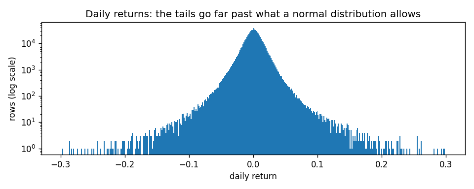

9. IC by year

Use it when: asked “is it one good year?”

ic_all = daily_ic(df, "signal")
by_year = ic_all.groupby(ic_all.index.year).mean()

fig, ax = plt.subplots(figsize=(6, 3.2))
ax.bar(by_year.index.astype(str), by_year.values, color=["C0" if v > 0 else "C3" for v in by_year.values])
ax.axhline(0, color="k", lw=0.8)
ax.set_ylabel("mean daily IC"); ax.set_title("Mean daily rank IC by calendar year")
fig.tight_layout()
fig.savefig("fig_by_year.png", dpi=120)
plt.show()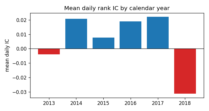

Many figures in a loop

This is the one block that keeps plt.close(fig). A loop that writes one PNG per signal, per year or per ticker should close each figure as soon as it is saved: every open figure holds its memory until the kernel stops, matplotlib warns once more than 20 are open, and a notebook draws every figure still open when the cell ends. The block writes files and shows nothing, on purpose; open the PNGs.

held = df.assign(rev5=-df.groupby("ticker")["close"].pct_change(5))
held = held[held["date"] > cut + embargo]
for name, col in (("1-day reversal", "signal"), ("5-day reversal", "rev5")):
    ic_c = daily_ic(held, col)
    fig, ax = plt.subplots(figsize=(8, 3.2))
    ic_c.cumsum().plot(ax=ax)
    ax.axhline(0, color="k", lw=0.8)
    ax.set_title("Cumulative daily rank IC, hold-out: %s (mean %+.4f)" % (name, ic_c.mean()))
    ax.set_ylabel("cumulative IC"); ax.set_xlabel("")
    fig.tight_layout()
    fig.savefig("fig_cum_ic_%s.png" % col, dpi=120)
    plt.close(fig)                        # inside a loop only: free each figure once it is on disk
    print("wrote fig_cum_ic_%s.png" % col)

wrote fig_cum_ic_signal.png
wrote fig_cum_ic_rev5.png

Habits

• fig.tight_layout() before savefig, or axis labels get clipped.
• Save, then show: fig.savefig(...) first, plt.show() last. plt.close(fig) belongs only in a loop that writes many files.
• Put the number in the title (“break-even at 2.4 bps”) so the chart stands on its own when it is pasted somewhere else.
• One chart per file, named for what it shows, regenerated by the same code that produced the numbers on the slide.

Which chart: stable? → rolling IC; survives? → build vs hold-out; is it big? → bps spread; how does it look over time? → cumulative IC; is it monotone? → deciles; what is the input? → histogram.