
A classifier that looks too good: the call-duration column
45,211 phone contacts from a bank's deposit campaigns, 11.7% of them successful. With the call's duration a logistic model reaches an AUC of 0.91; that column is only known after the outcome. Without it, 0.76. Then the accuracy trap on an 88/12 target, and what a chronological check shows when the base rate moves from 5% to 52%.
When a classifier scores far better than the problem seems to deserve, the first hypothesis is not that the problem was easy. It is that one column knows the answer. This study finds that column on a public marketing table, measures exactly how much it was worth, and then works through the two other traps the same table sets: an imbalanced target that makes accuracy meaningless, and a base rate that moves so much through time that the model’s probabilities stop meaning anything.
The data: direct-marketing phone contacts of a Portuguese bank between May 2008 and November 2010 (bank_marketing.csv, UCI repository): one row per contact, with the client’s age, job, marital status, education, balance and loans, how and when they were contacted, how many times, what happened in the previous campaign, and whether they subscribed to a term deposit.
The question, as it arrived: “Predict which clients will subscribe, so the next campaign can call the right people first.”
That last clause defines the prediction boundary. The prediction is used to decide whom to call; it is made before the call.
1. Understand the data
import pandas as pd, numpy as np

df = pd.read_csv("bank_marketing.csv", sep=";")
df["y"] = (df["y"] == "yes").astype(int)
print(df.shape, "| nulls:", int(df.isna().sum().sum()), "| duplicate rows:", df.duplicated().sum())
print("share subscribed: %.3f  (%d of %d)" % (df["y"].mean(), df["y"].sum(), len(df)))
print("'unknown' as a category:", {c: int((df[c] == "unknown").sum()) for c in ("job", "education", "contact", "poutcome")})
print(df[["age", "balance", "duration", "campaign", "pdays", "previous"]].describe().loc[["mean", "50%", "min", "max"]].round(1).to_string())
(45211, 17) | nulls: 0 | duplicate rows: 0
share subscribed: 0.117 (5289 of 45211)
'unknown' as a category: {'job': 288, 'education': 1857, 'contact': 13020, 'poutcome': 36959}
age balance duration campaign pdays previous
mean 40.9 1362.3 258.2 2.8 40.2 0.6
50% 39.0 448.0 180.0 2.0 -1.0 0.0
min 18.0 -8019.0 0.0 1.0 -1.0 0.0
max 95.0 102127.0 4918.0 63.0 871.0 275.0One row is one contact. No nulls, but “unknown” is a level of four categorical columns, which is missingness by another name (see missing values that mean something). Positives are 11.7% of rows. pdays is −1 for the 82% of clients never contacted before, a sentinel value that a linear model would read as a very small number of days.
There is no year column, but the documentation says the rows are in date order from May 2008 to November 2010. The month column wraps from December to January twice, which recovers the year:
months = ["jan", "feb", "mar", "apr", "may", "jun", "jul", "aug", "sep", "oct", "nov", "dec"]
df["m"] = df["month"].map({m: i for i, m in enumerate(months, 1)})
df["year"] = 2008 + (df["m"].diff().fillna(0) < 0).cumsum()     # the month number going backwards means a new year
print(df.groupby("year").agg(rows=("y", "size"), first_month=("month", "first"), last_month=("month", "last"), share_yes=("y", "mean")).round(3).to_string())
rows first_month last_month share_yes
year
2008 27729 may dec 0.051
2009 14862 jan dec 0.171
2010 2620 jan nov 0.516Three years, each much smaller than the last, and the share of successful calls goes from 5% to 17% to 52%. Keep that in mind for section 5.
2. The column that knows the answer
duration is the length of the last call in seconds. Its relationship with the outcome:
print("share subscribed by quartile of call duration:")
print(df.groupby(pd.qcut(df["duration"], 4))["y"].agg(["mean", "size"]).round(3).to_string())
print("calls under a minute: %d, subscribed %.4f | calls over ten minutes: %d, subscribed %.3f"
      % ((df["duration"] < 60).sum(), df.loc[df["duration"] < 60, "y"].mean(), (df["duration"] > 600).sum(), df.loc[df["duration"] > 600, "y"].mean()))
share subscribed by quartile of call duration:
mean size
duration
(-0.001, 103.0] 0.011 11375
(103.0, 180.0] 0.052 11285
(180.0, 319.0] 0.112 11290
(319.0, 4918.0] 0.294 11261
calls under a minute: 4659, subscribed 0.0019 | calls over ten minutes: 3790, subscribed 0.484Calls under a minute essentially never end in a subscription; calls over ten minutes end in one half the time. This is not a discovery about clients. A call in which the client says no is short, and a call in which the client goes through the paperwork is long. The duration is a consequence of the outcome, and it does not exist at the moment the decision to call is made. The documentation shipped with a later release of this dataset says the same: the column “should only be included for benchmark purposes and should be discarded if the intention is to have a realistic predictive model”.
Nothing about the column looks wrong in a summary table. It is numeric, complete, plausibly scaled. The only way to catch it is to ask, for each column, would this be known when the prediction is made? See prediction boundaries.
3. What the leak was worth
A logistic regression on one-hot categoricals and standardised numerics, with the scaler and the dummy columns learned on the training rows only. First the split a hurried analyst would use: random 70/30.
from sklearn.linear_model import LogisticRegression
from sklearn.metrics import roc_auc_score, average_precision_score, log_loss

cat = ["job", "marital", "education", "default", "housing", "loan", "contact", "month", "poutcome"]
num = ["age", "balance", "day", "campaign", "pdays", "previous"]

def design(d, num_cols, cat_cols, columns=None):
    parts = [d[num_cols].astype(float)]
    if cat_cols:
        parts.append(pd.get_dummies(d[cat_cols], dtype=float))
    X = pd.concat(parts, axis=1)
    return X if columns is None else X.reindex(columns=columns, fill_value=0.0)      # test frame gets the training columns

def evaluate(tr, te, num_cols, cat_cols, label):
    Xtr = design(tr, num_cols, cat_cols)
    Xte = design(te, num_cols, cat_cols, Xtr.columns)
    mu, sd = Xtr.mean(), Xtr.std().replace(0, 1)                      # learned on the training rows only
    model = LogisticRegression(max_iter=2000).fit(((Xtr - mu) / sd).values, tr["y"].values)
    p = model.predict_proba(((Xte - mu) / sd).values)[:, 1]
    y = te["y"].values
    print("%-36s AUC %.3f  PR-AUC %.3f  log-loss %.3f | accuracy at 0.5: %.3f (majority class: %.3f) | mean p %.3f, actual %.3f"
          % (label, roc_auc_score(y, p), average_precision_score(y, p), log_loss(y, p), ((p > 0.5) == y).mean(), max(y.mean(), 1 - y.mean()), p.mean(), y.mean()))
    return p

rng = np.random.RandomState(0)
idx = rng.permutation(len(df))
n_tr = int(0.7 * len(df))
tr, te = df.iloc[idx[:n_tr]], df.iloc[idx[n_tr:]]
print("random 70/30 split: %d train, %d test | log-loss of the constant base rate: %.3f" % (len(tr), len(te), log_loss(te["y"], np.full(len(te), tr["y"].mean()))))
p_leak = evaluate(tr, te, num + ["duration"], cat, "logistic, with duration")
p_dur = evaluate(tr, te, ["duration"], [], "logistic, duration only")
p_honest = evaluate(tr, te, num, cat, "logistic, without duration")
random 70/30 split: 31647 train, 13564 test | log-loss of the constant base rate: 0.366
logistic, with duration AUC 0.910 PR-AUC 0.584 log-loss 0.236 | accuracy at 0.5: 0.904 (majority class: 0.881) | mean p 0.116, actual 0.119
logistic, duration only AUC 0.815 PR-AUC 0.427 log-loss 0.300 | accuracy at 0.5: 0.890 (majority class: 0.881) | mean p 0.116, actual 0.119
logistic, without duration AUC 0.755 PR-AUC 0.405 log-loss 0.308 | accuracy at 0.5: 0.891 (majority class: 0.881) | mean p 0.117, actual 0.119With duration, AUC 0.91 and a log-loss well below the base rate. duration alone scores 0.82. Without it, 0.76. One column that cannot exist at prediction time is worth more than every other column combined.
Is 0.76 just a weak model? A gradient-boosted ensemble on the same honest columns:
from sklearn.ensemble import GradientBoostingClassifier

Xtr = design(tr, num, cat)
Xte = design(te, num, cat, Xtr.columns)
gbm = GradientBoostingClassifier(n_estimators=200, max_depth=3, random_state=0).fit(Xtr.values, tr["y"].values)
p_gbm = gbm.predict_proba(Xte.values)[:, 1]
y = te["y"].values
print("boosting, without duration           AUC %.3f  PR-AUC %.3f  log-loss %.3f" % (roc_auc_score(y, p_gbm), average_precision_score(y, p_gbm), log_loss(y, p_gbm)))
boosting, without duration AUC 0.793 PR-AUC 0.452 log-loss 0.291A more flexible model moves the honest number from 0.76 to 0.79. The leak moved it to 0.91. When a single column is worth more than a change of model class, the column is the thing to investigate, not the model. See debugging a model that looks too good.
4. The accuracy trap
Look again at the accuracy column above. The honest model scores 0.89 at a 0.5 threshold. Always predicting “no” scores 0.88. Those two numbers are the same story: with 12% positives, a model gains almost nothing in accuracy by being right about the positives, and a model that never predicts a positive is 88% accurate. Accuracy is the wrong instrument for this target.
from sklearn.metrics import precision_score, recall_score

print("honest logistic model, random split: what each threshold does")
for t in (0.5, 0.3, 0.2, 0.15, 0.1):
    flag = p_honest > t
    print("  threshold %.2f: flags %5.1f%% of clients | precision %.3f | recall %.3f | accuracy %.3f" % (t, 100 * flag.mean(), precision_score(y, flag), recall_score(y, flag), (flag == y).mean()))
honest logistic model, random split: what each threshold does
threshold 0.50: flags 3.3% of clients | precision 0.649 | recall 0.180 | accuracy 0.891
threshold 0.30: flags 7.2% of clients | precision 0.544 | recall 0.330 | accuracy 0.887
threshold 0.20: flags 11.1% of clients | precision 0.465 | recall 0.431 | accuracy 0.873
threshold 0.15: flags 17.4% of clients | precision 0.353 | recall 0.513 | accuracy 0.830
threshold 0.10: flags 37.7% of clients | precision 0.220 | recall 0.694 | accuracy 0.669At 0.5 the model flags 3% of clients and finds 18% of the subscribers. At 0.1 it flags 38% and finds 69%. Which is right depends on what a call costs and what a subscription is worth, and neither number appears in the table; the threshold is a business decision, and the model’s job is to produce a ranking and honest probabilities. That is why the scores reported above are AUC (ranking), PR-AUC (ranking, weighted toward the rare class) and log-loss (probabilities), not accuracy. See classification metrics.
Whether the probabilities are honest is a separate check:
dec = pd.qcut(p_honest, 10, labels=False, duplicates="drop")
cal = pd.DataFrame({"p": p_honest, "y": y}).groupby(dec).agg(mean_predicted=("p", "mean"), share_subscribed=("y", "mean"), n=("y", "size"))
print(cal.round(3).to_string())
mean_predicted share_subscribed n
0 0.018 0.032 1357
1 0.029 0.044 1356
2 0.046 0.060 1356
3 0.061 0.063 1357
4 0.074 0.066 1356
5 0.088 0.081 1356
6 0.105 0.086 1357
7 0.125 0.111 1356
8 0.168 0.162 1356
9 0.453 0.489 1357Under the random split the probabilities are usable: each decile’s mean prediction is close to its actual subscription rate. That is a property of the split as much as of the model, as the next section shows.
5. The chronological check
The purpose of the model is to be used on the next campaign. The honest test is to train on 2008 and 2009 and score 2010.
tr, te = df[df["year"] < 2010], df[df["year"] == 2010]
print("chronological split: train 2008-2009 (%d rows, %.1f%% yes), test 2010 (%d rows, %.1f%% yes)" % (len(tr), 100 * tr["y"].mean(), len(te), 100 * te["y"].mean()))
evaluate(tr, te, num + ["duration"], cat, "logistic, with duration")
evaluate(tr, te, num, cat, "logistic, without duration")
evaluate(tr, te, num, [c for c in cat if c != "month"], "logistic, without duration or month")
chronological split: train 2008-2009 (42591 rows, 9.2% yes), test 2010 (2620 rows, 51.6% yes)
logistic, with duration AUC 0.718 PR-AUC 0.706 log-loss 0.862 | accuracy at 0.5: 0.616 (majority class: 0.516) | mean p 0.313, actual 0.516
logistic, without duration AUC 0.662 PR-AUC 0.663 log-loss 0.862 | accuracy at 0.5: 0.569 (majority class: 0.516) | mean p 0.288, actual 0.516
logistic, without duration or month AUC 0.687 PR-AUC 0.691 log-loss 0.838 | accuracy at 0.5: 0.596 (majority class: 0.516) | mean p 0.260, actual 0.516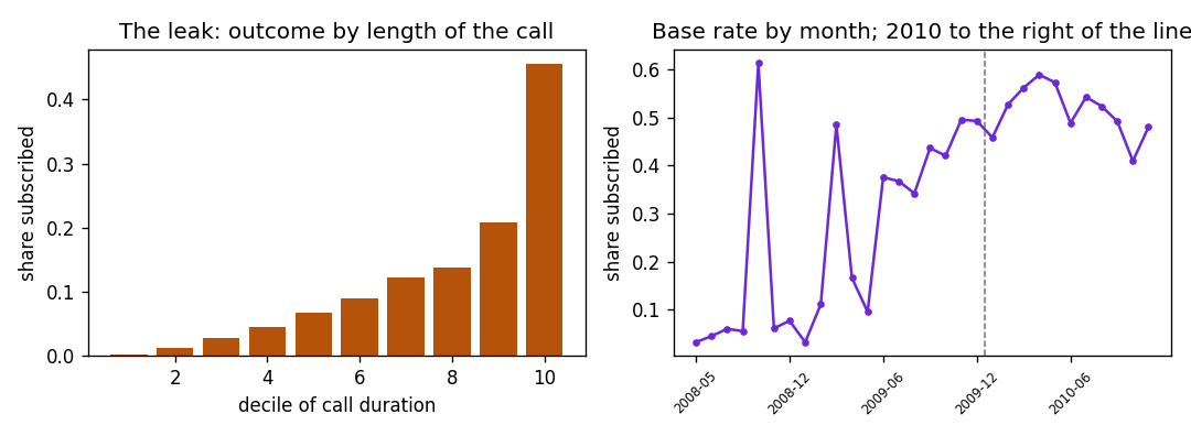
Show the code for this figure
import matplotlib.pyplot as plt

fig, (a1, a2) = plt.subplots(1, 2, figsize=(9, 3.3))
by_dur = df.groupby(pd.qcut(df["duration"], 10, labels=False, duplicates="drop"))["y"].mean()
a1.bar(by_dur.index + 1, by_dur.values, color="#b45309")
a1.set_xlabel("decile of call duration")
a1.set_ylabel("share subscribed")
a1.set_title("The leak: outcome by length of the call")
period = df["year"].astype(str) + "-" + df["m"].astype(str).str.zfill(2)
monthly = df.groupby(period)["y"].mean()
a2.plot(range(len(monthly)), monthly.values, marker="o", ms=3, color="#6d28d9")
a2.axvline(list(monthly.index).index("2010-01") - 0.5, color="#6b7280", ls="--", lw=0.9)
a2.set_xticks(range(0, len(monthly), 6))
a2.set_xticklabels(monthly.index[::6], rotation=45, fontsize=7)
a2.set_ylabel("share subscribed")
a2.set_title("Base rate by month; 2010 to the right of the line")
fig.tight_layout()
fig.savefig("bank-duration-leak-and-drift.png", dpi=120)
plt.show()
Three things changed. The ranking is weaker: AUC 0.66 without the leak, against 0.76 under the random split. The probabilities are wrong: the model expects 29% of the 2010 clients to subscribe and 52% do, because it learned a world where 9% did. And the month column now hurts: the model learned, from 2008 and 2009, that a May contact is a bad prospect (May 2008 was a huge low-yield campaign) and it applies that to a May 2010 in which most contacts succeeded. Dropping month improves the chronological AUC. A calendar column that encodes which campaign rather than which season is a leak of a subtler kind: it lets the model memorise the past rather than learn anything that transfers.
What changed in the campaigns themselves is visible in the columns:
print(pd.crosstab(df["year"], df["contact"], normalize="index").round(2).to_string())
print(pd.crosstab(df["year"], df["poutcome"], normalize="index").round(2).to_string())
contact cellular telephone unknown
year
2008 0.49 0.05 0.46
2009 0.91 0.09 0.00
2010 0.80 0.10 0.10
poutcome failure other success unknown
year
2008 0.03 0.01 0.00 0.97
2009 0.24 0.09 0.05 0.62
2010 0.24 0.13 0.29 0.34In 2008 nearly half the contacts had no recorded contact method and almost none had a previous-campaign outcome; by 2010 the bank was mostly calling mobiles and mostly calling people it had talked to before, nearly a third of whom had said yes last time. The 2010 rows are a different population, selected differently. The base rate did not drift on its own; the process that generates the rows changed. See distribution shift.
6. What to say
A logistic model predicts subscriptions with an AUC of 0.91 if it is given the length of the call, and 0.76 if it is not. The length of the call is determined by the outcome and is unknown when the decision to call is made, so 0.76 is the honest number under a random split, and a stronger model class only lifts it to 0.79. Accuracy is 0.89 against 0.88 for never predicting a subscription, so the model should be judged as a ranking (AUC, precision at the chosen call volume) and by its probabilities, which are well calibrated within the same period. Trained on 2008 and 2009 and applied to 2010, the ranking weakens to 0.66 and the probabilities are far too low, because the 2010 campaign targeted a different population with a success rate five times higher. Any model for the next campaign needs its base rate re-estimated, and should not use the month.
Takeaways
- A column that scores far above everything else is a suspect, not a find. Ask when it is recorded. Duration, a total that includes the outcome, a status field, a “date closed”: all are written after the event.
- The size of the jump is the tell. A better model class is worth a few points of AUC. A leak is worth fifteen.
- With a rare positive class, accuracy measures the base rate. Report the majority-class rate next to any accuracy, and prefer AUC, PR-AUC, log-loss and precision at a stated volume.
- The threshold is not a modelling choice. It comes from the cost of a call and the value of a subscription. Give the ranking and the calibration; let the decision-maker pick the point on the curve.
- A random split hides a moving base rate. If the model will be used later in time, test it later in time, and expect calibration to be the first casualty.
- Calendar columns can encode campaigns rather than seasons. If a “month” effect does not repeat across years, it is memorising, not learning.
Related: the taxi-tip column that contained the answer, leaked columns and labels that aren’t labels, and the hotel-cancellation study, where the post-event columns are less obvious and the threshold question is worked through in full.