Forecasting hourly electricity load: the naive forecasts are the competition

Load forecasting is the friendliest kind of forecasting: the series is smooth, the daily cycle is enormous, and yesterday is an excellent guide to today. That is precisely what makes it a good teaching case, because the naive forecasts are so strong that a model has to be judged against them, not against zero, and an R² of 0.97 can be a worse forecast than a one-line rule.

The data: electricity consumption for three distribution zones of a city, every ten minutes through 2017, with temperature, humidity and wind speed (tetouan_power.csv, UCI repository, Salam and El Hibaoui 2018). The three zones are summed into one city load.

The question, as it arrived: “Forecast the load.” At what horizon? Everything below depends on the answer, so two are used: one hour ahead and one day ahead (the same hour tomorrow).

1. Understand the data

import pandas as pd, numpy as np

raw = pd.read_csv("tetouan_power.csv")
raw.columns = [" ".join(c.split()) for c in raw.columns]        # two column names contain double spaces
raw["t"] = pd.to_datetime(raw["DateTime"])
zones = [c for c in raw.columns if "Power Consumption" in c]
raw["load"] = raw[zones].sum(axis=1) / 1000.0                    # total of the three zones, in MW
print(raw.shape, "| ten-minute rows from", raw["t"].min(), "to", raw["t"].max(), "| irregular steps:", int((raw["t"].diff().dt.total_seconds().dropna() != 600).sum()))
h = raw.set_index("t")[["load", "Temperature"]].resample("H").mean()
print("hourly rows:", len(h), "| nulls:", int(h.isna().sum().sum()))
print(h["load"].describe().round(1).to_string())
h["hour"], h["dow"], h["month"] = h.index.hour, h.index.dayofweek, h.index.month
print("mean load by hour:", h.groupby("hour")["load"].mean().round(0).astype(int).to_dict())
print("mean load by month:", h.groupby("month")["load"].mean().round(0).astype(int).to_dict())
print("mean load by weekday (0 = Monday):", h.groupby("dow")["load"].mean().round(1).to_dict())
print("correlation of hourly load with temperature: %.2f" % h["load"].corr(h["Temperature"]))

(52416, 11) | ten-minute rows from 2017-01-01 00:00:00 to 2017-12-30 23:50:00 | irregular steps: 0
hourly rows: 8736 | nulls: 0
count    8736.0
mean       71.2
std        17.0
min        37.4
25%        56.6
50%        69.9
75%        83.8
max       133.1
mean load by hour: {0: 69, 1: 62, 2: 59, 3: 57, 4: 55, 5: 52, 6: 50, 7: 51, 8: 57, 9: 64, 10: 70, 11: 74, 12: 76, 13: 76, 14: 75, 15: 74, 16: 73, 17: 77, 18: 86, 19: 96, 20: 98, 21: 95, 22: 88, 23: 78}
mean load by month: {1: 68, 2: 67, 3: 67, 4: 67, 5: 70, 6: 76, 7: 88, 8: 86, 9: 68, 10: 68, 11: 65, 12: 64}
mean load by weekday (0 = Monday): {0: 71.7, 1: 72.1, 2: 72.4, 3: 72.5, 4: 71.3, 5: 70.9, 6: 67.7}
correlation of hourly load with temperature: 0.49

One row is one hour, after resampling. A complete year with no gaps (the file ends a day early). The daily cycle runs from about 55 MW before dawn to nearly 100 MW at 8 pm; summer is 30% heavier than winter; the weekday effect is small; temperature correlates with load at about 0.5, which is the summer cooling load showing through.

2. The horizon decides the features

A lag is only usable if it is in the past of the target, not of the row. Lags are named here relative to the row’s own time $t$ : lag23 is the load 23 hours before $t$ . For a target one hour ahead ( $t+1$ ), lag23 is “the same hour yesterday” and lag167 is “the same hour last week”. For a target one day ahead ( $t+24$ ), the same hour yesterday is the current load, and the same hour last week is lag144. Getting this arithmetic wrong is the commonest way a forecasting page ends up scoring against the wrong baseline.

y = h["load"]
for k in (1, 2, 23, 24, 144, 167, 168):
    h["lag%d" % k] = y.shift(k)                     # load k hours before the row's own time t
h["ma24"] = y.shift(1).rolling(24).mean()           # mean of the 24 hours ending at t-1
h["ma168"] = y.shift(1).rolling(168).mean()
h["y1"] = y.shift(-1)                               # target A: the load one hour ahead
h["y24"] = y.shift(-24)                             # target B: the load at the same hour tomorrow
print(h.loc["2017-06-15 18:00":"2017-06-15 20:00", ["load", "lag1", "lag23", "lag167", "y1", "y24"]].round(1).to_string())

                      load   lag1  lag23  lag167     y1    y24
t                                                             
2017-06-15 18:00:00   85.3   79.9   99.3   100.4  100.2   85.5
2017-06-15 19:00:00  100.2   85.3  101.8   100.3  103.2   99.6
2017-06-15 20:00:00  103.2  100.2  100.5    98.4  100.7  101.6

Read one row: at 18:00 the current load is the value in load, y1 is the 19:00 value on the next line, y24 is 18:00 tomorrow. Print three rows like this for every new target; see forward targets and look-ahead leakage.

Temperature is used as the current temperature. A day-ahead forecast would only have a weather forecast, so including it is generous to the model; it turns out not to matter.

3. Split and baselines

Chronological: the last quarter of the year is the test period. The baselines are the naive forecasts a dispatcher would use without a model.

test_start = pd.Timestamp("2017-10-01")
te = h[h.index >= test_start]

def r2(y, yhat):
    return 1 - np.sum((y - yhat) ** 2) / np.sum((y - y.mean()) ** 2)

def mae(y, yhat):
    return np.mean(np.abs(y - yhat))

def score(label, actual, pred):
    ok = ~(np.isnan(actual) | np.isnan(pred))
    print("%-58s R2 %.3f  MAE %5.2f MW" % (label, r2(actual[ok], pred[ok]), mae(actual[ok], pred[ok])))

print("test period: %s -> %s, %d hours" % (te.index.min(), te.index.max(), len(te)))
print("--- one hour ahead")
score("naive: the current hour", te["y1"].values, te["load"].values)
score("naive: the same hour yesterday", te["y1"].values, te["lag23"].values)
score("naive: the same hour last week", te["y1"].values, te["lag167"].values)
print("--- one day ahead")
score("naive: the same hour today", te["y24"].values, te["load"].values)
score("naive: the same hour last week", te["y24"].values, te["lag144"].values)
clim = h[h.index < test_start].groupby(["hour", "dow"])["load"].mean()
score("train mean by hour x weekday", te["y24"].values, pd.Series(list(zip(te["hour"], te["dow"]))).map(clim).values)

test period: 2017-10-01 00:00:00 -> 2017-12-30 23:00:00, 2184 hours
--- one hour ahead
naive: the current hour                                    R2 0.838  MAE  4.06 MW
naive: the same hour yesterday                             R2 0.949  MAE  2.03 MW
naive: the same hour last week                             R2 0.965  MAE  1.87 MW
--- one day ahead
naive: the same hour today                                 R2 0.949  MAE  2.03 MW
naive: the same hour last week                             R2 0.965  MAE  1.87 MW
train mean by hour x weekday                               R2 0.484  MAE  8.77 MW

“Same hour last week” scores an R² of 0.965 at both horizons with an error under 2 MW on a 70 MW load. That is the number to beat. Note what the R² column does here: persistence one hour ahead scores 0.84 and is the worst forecast in the table. On a series with a strong cycle, R² is dominated by the cycle and says almost nothing about forecast quality; the error in the series’ own units against the naive is what to report. The calendar-cell mean, which is what a model without lags amounts to, is far behind.

4. A ridge regression on lags and calendar dummies

One-hot hour and weekday, plus the lags appropriate to the horizon, fitted on January to September.

from sklearn.linear_model import Ridge

cal = pd.get_dummies(h["hour"].astype(str), prefix="h", dtype=float).join(pd.get_dummies(h["dow"].astype(str), prefix="d", dtype=float))

def fit_score(target, feats, label, model=None):
    d = h.dropna(subset=feats + [target])
    X = pd.concat([d[feats], cal.loc[d.index]], axis=1).values
    tr = d.index < test_start
    m = (model if model is not None else Ridge(alpha=1.0)).fit(X[tr], d[target].values[tr])
    score(label, d[target].values[~tr], m.predict(X[~tr]))

print("--- one hour ahead")
fit_score("y1", ["load"], "ridge: current load + hour and weekday dummies")
fit_score("y1", ["load", "lag1", "lag2", "lag23", "lag167"], "ridge: + lags 1, 2, 23, 167")
fit_score("y1", ["load", "lag1", "lag2", "lag23", "lag167", "Temperature"], "ridge: + current temperature")
print("--- one day ahead")
fit_score("y24", ["load"], "ridge: current load + hour and weekday dummies")
fit_score("y24", ["load", "lag24", "lag144", "lag168"], "ridge: + lags 24, 144, 168")
fit_score("y24", ["load", "lag24", "lag144", "lag168", "ma24", "ma168"], "ridge: + trailing 24h and 168h means")
fit_score("y24", ["load", "lag24", "lag144", "lag168", "ma24", "ma168", "Temperature"], "ridge: + current temperature")

--- one hour ahead
ridge: current load + hour and weekday dummies             R2 0.901  MAE  2.72 MW
ridge: + lags 1, 2, 23, 167                                R2 0.975  MAE  1.56 MW
ridge: + current temperature                               R2 0.975  MAE  1.56 MW
--- one day ahead
ridge: current load + hour and weekday dummies             R2 0.972  MAE  1.66 MW
ridge: + lags 24, 144, 168                                 R2 0.979  MAE  1.44 MW
ridge: + trailing 24h and 168h means                       R2 0.979  MAE  1.45 MW
ridge: + current temperature                               R2 0.979  MAE  1.45 MW

With the right lags the ridge is at 1.56 MW an hour ahead and 1.44 MW a day ahead, against 1.87 for the best naive: about 20% less error. Everything after that is a null result worth stating plainly. Trailing means add nothing the lags did not already carry. The current temperature adds nothing either, which is not because load is unrelated to temperature (the correlation is 0.5) but because the lags already contain the temperature’s effect on yesterday’s and last week’s load, and a day-to-day temperature change is not large enough to matter on top.

A forest on the same columns:

from sklearn.ensemble import RandomForestRegressor

fit_score("y1", ["load", "lag1", "lag2", "lag23", "lag167"], "forest: lags 1, 2, 23, 167 + calendar (one hour ahead)",
          RandomForestRegressor(n_estimators=100, min_samples_leaf=3, random_state=0, n_jobs=-1))
fit_score("y24", ["load", "lag24", "lag144", "lag168", "ma24", "ma168"], "forest: lags + trailing means + calendar (one day ahead)",
          RandomForestRegressor(n_estimators=100, min_samples_leaf=3, random_state=0, n_jobs=-1))

forest: lags 1, 2, 23, 167 + calendar (one hour ahead)     R2 0.982  MAE  1.28 MW
forest: lags + trailing means + calendar (one day ahead)   R2 0.977  MAE  1.46 MW

The forest helps an hour ahead (1.28 MW), where the very recent lags carry a nonlinear signal about the current ramp, and not a day ahead. Neither result changes the conclusion: the model is worth roughly a fifth to a third of the naive error, and no more.

5. Walk-forward: does the edge hold every month?

A single split can be lucky. Refit the day-ahead ridge at the start of every month from April, on all data to date, and score that month.

feats = ["load", "lag24", "lag144", "lag168", "ma24", "ma168"]
d = h.dropna(subset=feats + ["y24"])
X = pd.concat([d[feats], cal.loc[d.index]], axis=1).values
rows, preds = [], {}
for month in range(4, 13):
    tr = d.index < pd.Timestamp("2017-%02d-01" % month)
    te_m = d.index.month == month
    p = Ridge(alpha=1.0).fit(X[tr], d["y24"].values[tr]).predict(X[te_m])
    preds[month] = pd.Series(p, index=d.index[te_m])
    actual = d["y24"].values[te_m]
    rows.append((month, mae(actual, p), mae(actual, d["lag144"].values[te_m]), mae(actual, d["load"].values[te_m])))
wf = pd.DataFrame(rows, columns=["month", "ridge", "naive: last week", "naive: today"]).set_index("month")
print(wf.round(2).to_string())
print("ridge error as a share of the last-week naive, averaged over months: %.2f" % (wf["ridge"] / wf["naive: last week"]).mean())

       ridge  naive: last week  naive: today
month                                       
4       1.25              1.70          2.17
5       1.91              2.75          2.28
6       2.11              3.50          2.50
7       2.48              5.50          2.86
8       2.65              5.13          2.59
9       2.10              4.15          2.50
10      1.16              1.45          1.89
11      1.84              2.53          2.29
12      1.32              1.65          1.90
ridge error as a share of the last-week naive, averaged over months: 0.65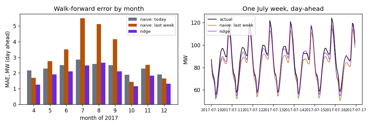

Monthly day-ahead error of the ridge against the two naive forecasts, and one July week of actual load against the last-week naive and the model

Show the code for this figure

import matplotlib.pyplot as plt

fig, (a1, a2) = plt.subplots(1, 2, figsize=(10, 3.4))
x = np.arange(len(wf))
a1.bar(x - 0.27, wf["naive: today"], 0.27, label="naive: today", color="#6b7280")
a1.bar(x, wf["naive: last week"], 0.27, label="naive: last week", color="#b45309")
a1.bar(x + 0.27, wf["ridge"], 0.27, label="ridge", color="#6d28d9")
a1.set_xticks(x)
a1.set_xticklabels(wf.index)
a1.set_xlabel("month of 2017")
a1.set_ylabel("MAE, MW (day ahead)")
a1.set_title("Walk-forward error by month")
a1.legend(fontsize=8)
week = slice("2017-07-10", "2017-07-16")
shifted = d["y24"].shift(24, freq="H")                      # put each target back at the hour it describes
a2.plot(shifted[week].index, shifted[week].values, color="k", lw=1.2, label="actual")
a2.plot(d["lag144"].shift(24, freq="H")[week].index, d["lag144"].shift(24, freq="H")[week].values, color="#b45309", lw=0.9, label="naive: last week")
a2.plot(preds[7].shift(24, freq="H")[week].index, preds[7].shift(24, freq="H")[week].values, color="#6d28d9", lw=0.9, label="ridge")
a2.set_title("One July week, day-ahead")
a2.set_ylabel("MW")
a2.tick_params(axis="x", labelsize=7)
a2.legend(fontsize=8)
fig.tight_layout()
fig.savefig("tetouan-walk-forward.png", dpi=120)
plt.show()

The ridge beats the last-week naive in every one of nine months, by most in July and August, when the load level moves from week to week with the heat and “same hour last week” is a poor guide. In those months “same hour today” is the better naive, and in August it edges the model (2.59 against 2.65 MW). In the flat months the last-week naive is within about half a megawatt of the model.

6. What to say

The load has a daily cycle that dwarfs everything else, so “the same hour last week” forecasts it with a mean error of 1.9 MW on a 70 MW load, an hour or a day ahead. A ridge regression on lagged loads and hour and weekday dummies brings that to 1.4 to 1.6 MW, and beats the naive in every month of a walk-forward test, by most in summer when the level shifts week to week. Temperature and trailing averages add nothing once the lags are in; a forest helps only at the one-hour horizon. Reported honestly, the model removes between a fifth and a third of the naive forecast’s error, depending on the month.

Takeaways

Name the horizon first. The feature set, the baseline and the score all depend on it, and a page that does not say “one hour ahead” is not reporting a forecast.
Build lags relative to the target’s time, and print three rows to check. The same-hour-last-week lag is 167 for one horizon and 144 for the other.
The seasonal naive is the baseline. On a cyclical series it will score an R² in the high nineties; report the error in the series’ own units and the model’s error as a share of the naive’s.
R² on a cyclical series measures the cycle. Persistence scored 0.84 and was the worst forecast in the table.
Null results are results. Temperature and trailing means did nothing here; saying so is more useful than a table where every row is a little better than the last.
Walk forward before believing a single split. Nine wins in nine months against the last-week naive is the evidence, and the one month where the other naive wins is part of it; one quarter is a hint.

For a series where the level drifts and the same comparison comes out differently, see hourly bike rentals; for a traffic series with a messier clock, traffic volume against a seasonal baseline; for the version of the horizon question on financial signals, feature decay across horizons.