
Hotel cancellations: duplicates, post-booking columns and the threshold
119,390 bookings at two hotels, 37% of them cancelled. A forest scores an AUC of 0.88 on a shuffled split; a quarter of the rows are exact duplicates and four columns are written after the booking. With those handled and a chronological test, 0.74. Then what the probabilities are for, which is a decision, not a score.
Cancellation prediction is a well-behaved problem on paper: a binary target with a healthy positive rate, a few dozen columns, a hundred thousand rows. This study is about the three things that make the first number wrong on this particular table, and then about what the right number is for, because a probability of cancellation is only useful if someone decides something with it.
The data: bookings at a city hotel and a resort hotel in Portugal with arrivals between July 2015 and August 2017 (hotel_bookings.csv, published with Antonio, de Almeida and Nunes, Data in Brief, 2019). One row per booking: when it was made and for when, the party, the channel it came through, the deposit terms, the rate, and whether it was cancelled.
The question, as it arrived: “Predict which bookings will cancel.” The prediction is made at booking time, or at least well before arrival, because that is when it can change what the hotel does.
1. Understand the data
import pandas as pd, numpy as np

df = pd.read_csv("hotel_bookings.csv")
df["arrival"] = pd.to_datetime(df["arrival_date_year"].astype(str) + "-" + df["arrival_date_month"] + "-" + df["arrival_date_day_of_month"].astype(str), format="%Y-%B-%d")
print(df.shape, "| arrivals", df["arrival"].min().date(), "->", df["arrival"].max().date())
print("cancelled: %.3f | by hotel:" % df["is_canceled"].mean(), df.groupby("hotel")["is_canceled"].mean().round(3).to_dict())
print("nulls:", df.isna().sum()[lambda s: s > 0].to_dict())
print("exact duplicate rows: %d (%.1f%%)" % (df.duplicated().sum(), 100 * df.duplicated().mean()))
print(pd.crosstab(df["reservation_status"], df["is_canceled"]))
(119390, 33) | arrivals 2015-07-01 -> 2017-08-31
cancelled: 0.370 | by hotel: {'City Hotel': 0.417, 'Resort Hotel': 0.278}
nulls: {'children': 4, 'country': 488, 'agent': 16340, 'company': 112593}
exact duplicate rows: 31994 (26.8%)
is_canceled 0 1
reservation_status
Canceled 0 43017
Check-Out 75166 0
No-Show 0 1207One row is one booking. Two obvious things and one that is not. reservation_status is the target with three labels instead of two (it and its date are excluded from everything). agent and company are mostly null, which here means “no agent” and “no company”: absence with a meaning, not a recording failure. And a quarter of the rows are exact copies of another row, which is the subject of section 3.
2. The prediction boundary
Most columns describe the booking as it was made. Four describe what happened to it afterwards:
print("cancel rate by required_car_parking_spaces:", df.groupby(df["required_car_parking_spaces"].clip(upper=1))["is_canceled"].agg(["mean", "size"]).round(3).to_dict())
differ = df["assigned_room_type"] != df["reserved_room_type"]
print("cancel rate when the assigned room differs from the reserved one: %.3f (%.1f%% of bookings) vs %.3f when it is the same" % (df.loc[differ, "is_canceled"].mean(), 100 * differ.mean(), df.loc[~differ, "is_canceled"].mean()))
print("cancel rate by booking_changes:", df.groupby(df["booking_changes"].clip(upper=2))["is_canceled"].mean().round(3).to_dict())
print("cancel rate by total_of_special_requests:", df.groupby(df["total_of_special_requests"].clip(upper=3))["is_canceled"].mean().round(3).to_dict())
cancel rate by required_car_parking_spaces: {'mean': {0: 0.395, 1: 0.0}, 'size': {0: 111974, 1: 7416}}
cancel rate when the assigned room differs from the reserved one: 0.054 (12.5% of bookings) vs 0.416 when it is the same
cancel rate by booking_changes: {0: 0.409, 1: 0.142, 2: 0.191}
cancel rate by total_of_special_requests: {0: 0.477, 1: 0.22, 2: 0.221, 3: 0.168}Nobody with a parking space cancelled: not a single booking out of seven thousand. Parking is recorded at check-in, so having one means the guest arrived. A room assigned differently from the one reserved is likewise something that happens at check-in, and those bookings cancel at 5%. Booking changes and special requests accumulate over the life of the booking and are strongly associated with not cancelling, partly because a guest who is going to cancel does not phone to ask for a cot. None of these four columns is available at the moment the question is being asked. They are kept out of the honest feature set and put back once, in section 4, to measure what they were worth. See prediction boundaries; the same trap in a much more obvious costume is the call-duration column.
3. Duplicates
twin = df.duplicated(keep=False)
print("rows with at least one exact twin: %.1f%% | cancel rate among them %.3f, among the rest %.3f" % (100 * twin.mean(), df.loc[twin, "is_canceled"].mean(), df.loc[~twin, "is_canceled"].mean()))
print("twins by deposit type:", df.loc[twin, "deposit_type"].value_counts(normalize=True).round(3).to_dict())
print("twins by market segment:", df.loc[twin, "market_segment"].value_counts(normalize=True).round(3).head(3).to_dict())
dd = df.drop_duplicates().reset_index(drop=True)
print("after dropping duplicates: %d rows, cancel rate %.3f" % (len(dd), dd["is_canceled"].mean()))
rows with at least one exact twin: 33.6% | cancel rate among them 0.584, among the rest 0.262
twins by deposit type: {'No Deposit': 0.642, 'Non Refund': 0.356, 'Refundable': 0.002}
twins by market segment: {'Groups': 0.416, 'Offline TA/TO': 0.304, 'Online TA': 0.206}
after dropping duplicates: 87396 rows, cancel rate 0.275A third of the rows have an identical twin, and the twins cancel at more than twice the rate of the rest. Many are group and tour-operator bookings entered as one row per room, all with the same attributes, and when the group cancels every row cancels. For a model this is the worst kind of repetition: under a random split, most of a group’s rows land in training and the rest in test, and the model scores by recognising the group, not by predicting anything. The rest of this study uses the deduplicated table. That is a decision with a cost, since a group of ten identical rooms is a real thing, but it is the decision that makes the evaluation honest; a row count is not the same as an evidence count. See check 3 in leaked columns and labels.
4. Validation, and what the first two traps were worth
Chronological by arrival date, with the 2017 arrivals as the test period, on the deduplicated table. First, the same forest under the splits a hurried analysis would use, to see how far each trap moves the number.
from sklearn.linear_model import LogisticRegression
from sklearn.ensemble import RandomForestClassifier
from sklearn.metrics import roc_auc_score, average_precision_score, log_loss

at_booking = ["hotel", "lead_time", "arrival_date_month", "arrival_date_week_number", "stays_in_weekend_nights", "stays_in_week_nights",
              "adults", "children", "babies", "meal", "market_segment", "distribution_channel", "is_repeated_guest",
              "previous_cancellations", "previous_bookings_not_canceled", "reserved_room_type", "deposit_type", "customer_type", "adr", "days_in_waiting_list"]
after_booking = ["booking_changes", "total_of_special_requests", "assigned_room_type", "required_car_parking_spaces"]
categorical = ["hotel", "arrival_date_month", "meal", "market_segment", "distribution_channel", "reserved_room_type", "deposit_type", "customer_type", "assigned_room_type"]

def design(d, cols, columns=None):
    num = [c for c in cols if c not in categorical]
    cat = [c for c in cols if c in categorical]
    X = pd.concat([d[num].astype(float).fillna(0.0), pd.get_dummies(d[cat].astype(str), dtype=float)], axis=1)
    return X if columns is None else X.reindex(columns=columns, fill_value=0.0)

def evaluate(tr, te, cols, label, model="forest"):
    Xtr = design(tr, cols)
    Xte = design(te, cols, Xtr.columns)
    if model == "logistic":
        mu, sd = Xtr.mean(), Xtr.std().replace(0, 1)
        m = LogisticRegression(max_iter=3000).fit(((Xtr - mu) / sd).values, tr["is_canceled"].values)
        p = m.predict_proba(((Xte - mu) / sd).values)[:, 1]
    else:
        m = RandomForestClassifier(n_estimators=100, min_samples_leaf=5, random_state=0, n_jobs=-1).fit(Xtr.values, tr["is_canceled"].values)
        p = m.predict_proba(Xte.values)[:, 1]
    y = te["is_canceled"].values
    print("%-58s AUC %.3f  PR-AUC %.3f  log-loss %.3f | mean p %.3f, actual %.3f" % (label, roc_auc_score(y, p), average_precision_score(y, p), log_loss(y, p), p.mean(), y.mean()))
    return p

rng = np.random.RandomState(0)
def random_split(d):
    idx = rng.permutation(len(d))
    n = int(0.7 * len(d))
    return d.iloc[idx[:n]], d.iloc[idx[n:]]

tr, te = random_split(df)
evaluate(tr, te, at_booking, "random split, duplicates kept: forest")
tr, te = random_split(dd)
evaluate(tr, te, at_booking, "random split, duplicates dropped: forest")
tr, te = dd[dd["arrival"] < "2017-01-01"], dd[dd["arrival"] >= "2017-01-01"]
print("chronological: %d bookings arriving before 2017 (cancel rate %.3f) -> %d arriving in 2017 (cancel rate %.3f)" % (len(tr), tr["is_canceled"].mean(), len(te), te["is_canceled"].mean()))
p_lr = evaluate(tr, te, at_booking, "chronological, deduplicated: logistic", "logistic")
p_rf = evaluate(tr, te, at_booking, "chronological, deduplicated: forest")
evaluate(tr, te, at_booking + after_booking, "chronological, deduplicated: forest + post-booking columns")
evaluate(tr, te, [c for c in at_booking if c != "deposit_type"], "chronological, deduplicated: forest without deposit_type")
random split, duplicates kept: forest AUC 0.884 PR-AUC 0.853 log-loss 0.395 | mean p 0.371, actual 0.369
random split, duplicates dropped: forest AUC 0.788 PR-AUC 0.606 log-loss 0.475 | mean p 0.272, actual 0.275
chronological: 55704 bookings arriving before 2017 (cancel rate 0.250) -> 31692 arriving in 2017 (cancel rate 0.319)
chronological, deduplicated: logistic AUC 0.727 PR-AUC 0.559 log-loss 0.553 | mean p 0.302, actual 0.319
chronological, deduplicated: forest AUC 0.744 PR-AUC 0.565 log-loss 0.539 | mean p 0.290, actual 0.319
chronological, deduplicated: forest + post-booking columns AUC 0.798 PR-AUC 0.633 log-loss 0.503 | mean p 0.291, actual 0.319
chronological, deduplicated: forest without deposit_type AUC 0.741 PR-AUC 0.550 log-loss 0.545 | mean p 0.292, actual 0.319The same forest on the same at-booking columns: 0.88 with the duplicates in and a shuffled split, 0.79 with the duplicates out, 0.74 tested on the following year. The first number is mostly memorised twins. Putting the four post-booking columns back adds five points of AUC that would not exist in use. Two traps, each worth several times the difference between a logistic regression and a forest on the honest columns.
The test period also has a higher cancellation rate than the training period, and the forest’s mean probability is below it. That gap reappears in the calibration table below.
5. Baselines, and a feature that is not what it seems
y = te["is_canceled"].values
print("majority class accuracy on the 2017 bookings: %.3f | log-loss of the constant training rate: %.3f" % (max(y.mean(), 1 - y.mean()), log_loss(y, np.full(len(y), tr["is_canceled"].mean()))))
for c in ("lead_time", "previous_cancellations", "adr"):
    print("single column %-28s AUC %.3f" % (c, roc_auc_score(y, te[c].values)))
seg = te["market_segment"].map(tr.groupby("market_segment")["is_canceled"].mean()).fillna(tr["is_canceled"].mean())
print("single column %-28s AUC %.3f" % ("market_segment (train rate)", roc_auc_score(y, seg.values)))
majority class accuracy on the 2017 bookings: 0.681 | log-loss of the constant training rate: 0.638
single column lead_time AUC 0.648
single column previous_cancellations AUC 0.497
single column adr AUC 0.589
single column market_segment (train rate) AUC 0.619Lead time alone ranks bookings at 0.65: the further ahead a booking is made, the more likely it is to be cancelled. The forest’s 0.74 is against that, not against 0.5.
The column everyone notices first in this table is the deposit type, because a non-refundable deposit is associated with cancelling almost every time, which is the opposite of what a deposit is for:
print("deposit_type, all rows:")
print(df.groupby("deposit_type")["is_canceled"].agg(["mean", "size"]).round(3).to_string())
print("deposit_type, deduplicated:")
print(dd.groupby("deposit_type")["is_canceled"].agg(["mean", "size"]).round(3).to_string())
nr = df[df["deposit_type"] == "Non Refund"]
print("Non Refund rows: %.1f%% have an exact twin | by market segment:" % (100 * nr.duplicated(keep=False).mean()), nr["market_segment"].value_counts(normalize=True).round(2).head(3).to_dict())
deposit_type, all rows:
mean size
deposit_type
No Deposit 0.284 104641
Non Refund 0.994 14587
Refundable 0.222 162
deposit_type, deduplicated:
mean size
deposit_type
No Deposit 0.267 86251
Non Refund 0.947 1038
Refundable 0.243 107
Non Refund rows: 98.1% have an exact twin | by market segment: {'Groups': 0.63, 'Offline TA/TO': 0.34, 'Corporate': 0.02}The pattern is real in the file, but it lives in the duplicated rows: the non-refundable bookings are overwhelmingly group and tour-operator blocks, entered as one row per room, that were cancelled as a block. After deduplication there are far fewer of them, and in section 4 removing the column from the forest barely moved the chronological AUC. A feature whose entire effect sits inside repeated rows is a feature about how the data was entered. It may or may not describe the next year’s bookings; the honest test says it is not carrying much.
6. Calibration and the threshold
The forest’s probabilities, by decile, against what actually happened in 2017:
from sklearn.metrics import precision_score, recall_score

dec = pd.qcut(p_rf, 10, labels=False, duplicates="drop")
cal = pd.DataFrame({"p": p_rf, "y": y}).groupby(dec).agg(mean_predicted=("p", "mean"), cancel_rate=("y", "mean"), n=("y", "size"))
print(cal.round(3).to_string())
print("threshold  flagged  precision  recall")
for t in (0.3, 0.4, 0.5, 0.6, 0.7):
    flag = p_rf > t
    print("   %.1f     %5.1f%%    %.3f     %.3f" % (t, 100 * flag.mean(), precision_score(y, flag), recall_score(y, flag)))
mean_predicted cancel_rate n
0 0.057 0.059 3170
1 0.106 0.107 3173
2 0.142 0.145 3165
3 0.186 0.171 3171
4 0.260 0.270 3167
5 0.335 0.398 3169
6 0.379 0.445 3169
7 0.413 0.464 3169
8 0.453 0.507 3169
9 0.569 0.627 3170
threshold flagged precision recall
0.3 50.7% 0.485 0.771
0.4 28.8% 0.536 0.483
0.5 6.8% 0.675 0.145
0.6 1.7% 0.901 0.049
0.7 1.1% 0.991 0.033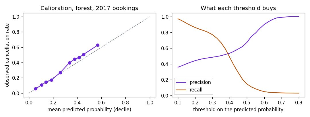
Show the code for this figure
import matplotlib.pyplot as plt

fig, (a1, a2) = plt.subplots(1, 2, figsize=(9, 3.4))
a1.plot([0, 1], [0, 1], color="#6b7280", lw=0.8, ls="--")
a1.plot(cal["mean_predicted"], cal["cancel_rate"], marker="o", color="#6d28d9")
a1.set_xlabel("mean predicted probability (decile)")
a1.set_ylabel("observed cancellation rate")
a1.set_title("Calibration, forest, 2017 bookings")
ts = np.linspace(0.1, 0.8, 29)
prec = [precision_score(y, p_rf > t) for t in ts]
rec = [recall_score(y, p_rf > t) for t in ts]
a2.plot(ts, prec, label="precision", color="#6d28d9")
a2.plot(ts, rec, label="recall", color="#b45309")
a2.set_xlabel("threshold on the predicted probability")
a2.set_title("What each threshold buys")
a2.legend()
fig.tight_layout()
fig.savefig("hotel-calibration-threshold.png", dpi=120)
plt.show()
The ranking is honest: each decile cancels more often than the one below. The level is slightly off, with the upper deciles cancelling more than predicted, which is the 2017 rate being higher than the training rate. If the probabilities are going to be used as probabilities (for expected occupancy, say), that offset has to be corrected, and it will drift again next year.
The threshold is the part of this problem that is not statistics. At 0.5 the model flags 7% of bookings and is right about two-thirds of them, catching 15% of the cancellations. At 0.3 it flags half of all bookings and catches three-quarters of the cancellations, being right about half the time. Which is better depends entirely on what a flag triggers. Suppose, for illustration only, a flagged booking gets a confirmation call that costs one unit, and a cancellation found early is worth five. Then a call pays off whenever precision exceeds 0.2, every threshold in the table clears that, and the hotel should flag at 0.3 and phone half its guests. Change the value of an early catch to two units and the break-even precision is 0.5, and 0.4 becomes the threshold. The model does not know those numbers. Its job is the ranking and the calibration; the threshold is chosen by whoever owns the costs. See classification metrics.
7. What to say
A forest on the columns known at booking time predicts cancellations with an AUC of 0.74 on the following year’s arrivals, against 0.65 for lead time alone. The 0.88 that a shuffled split reports is mostly the model recognising the quarter of rows that are exact duplicates of each other, and the four columns recorded after booking (parking, assigned room, changes, requests) would add another five points that do not exist when the prediction is needed. The probabilities rank well and run a little low against 2017’s higher cancellation rate. Whether to act on a booking is a threshold decision that depends on what a flag costs and what an early catch is worth; at a threshold of 0.3 the model flags half the bookings and finds three-quarters of the cancellations.
Takeaways
- Count exact duplicates before anything else, and find out what they are. Twins across train and test turn any model into a lookup table, and a random split guarantees twins.
- Post-event columns can look like ordinary attributes. Parking spaces, assigned rooms, changes and requests are all plausible features. The question is not “is this predictive” but “when is this written”.
- A striking single-column pattern deserves a duplicate check. The non-refundable-deposit effect was real in the file and lived almost entirely in repeated rows.
- Report the ranking, the calibration, and the trade-off curve. The threshold belongs to whoever owns the costs; give them the curve, not a point on it.
- Calibration drifts with the base rate. Test on a later period and expect the level to be off before the ranking is.
Related: the bank marketing study, where the leak is one obvious column and the class is rare; the flight-delay study, where the prediction boundary moves and the feature set moves with it.