
Does relative volume predict the size of tomorrow's move?
A second complete pass on the same public file, with a different kind of question. Both quantities had to be defined precisely before anything could be scored, and the boring explanation had to be scored alongside the interesting one.
Same file as the reversal study, different question, and a different lesson: this time the work was in defining the two quantities and in naming the dull mechanism that had to be beaten. Every number on this page comes from the code on it.
The question, as it arrived: “Does yesterday’s volume tell you anything about the size of tomorrow’s move?”
1. Turning it into a question a number can answer
The brief has two undefined terms, and both needed a decision before any code.
“Yesterday’s volume.” Raw volume differs a hundredfold across tickers; a busy day for a utility is a quiet one for a semiconductor. So the reading has to be per ticker, relative to that ticker’s own recent history. Exactly how is a choice: volume over its trailing average, a z-score, or its rank within the ticker’s own history. I chose the ratio to the trailing 20-day mean, because it is the simplest to explain.
“The size of tomorrow’s move.” Absolute return tomorrow? High minus low over close? And raw, or relative to how much that stock normally moves? A stock that moves 3% a day will always look “big” next to one that moves 0.5%. So: tomorrow’s absolute close-to-close return, divided by the stock’s trailing 20-day volatility. “How big was tomorrow, relative to normal for this stock.”
The boring explanation. If high volume today predicts a big move tomorrow, what is the dull mechanism? Volatility clusters: a big move today predicts a big move tomorrow, and busy days are big-move days. Volume may be predicting tomorrow only by proxying for today’s move. The baseline is therefore not zero; it is today’s normalised move size, and the protocol commits to scoring it under the same rules. See does a signal add anything beyond a baseline?.
2. Data decisions
The interrogation is the same file, so the same three findings and the same decisions: drop the 22 short histories, keep the 46 extreme moves and use ranks, flag survivorship (less of a concern for a volatility question than for a return question, but still said).
import pandas as pd, numpy as np

df = pd.read_csv("all_stocks_5yr.csv")
df["date"] = pd.to_datetime(df["date"])
df = df.rename(columns={"Name": "ticker"}).sort_values(["ticker", "date"]).reset_index(drop=True)
per = df.groupby("ticker").size()
df = df[df["ticker"].isin(per[per >= 1000].index)].copy()
g = df.groupby("ticker")

df["ret"] = g["close"].pct_change()
df["vol20"] = g["ret"].transform(lambda x: x.rolling(20).std())
df["target"] = g["ret"].shift(-1).abs() / df["vol20"]                                 # tomorrow's move, in units of own vol
df["relvol"] = df["volume"] / g["volume"].transform(lambda x: x.rolling(20).mean())   # today's volume relative to own normal
df["base"] = df["ret"].abs() / df["vol20"]                                             # today's move, in units of own vol
df = df.replace([np.inf, -np.inf], np.nan).dropna(subset=["target", "relvol", "base"])

print(len(df), "rows | target: median %.3f  mean %.3f  max %.1f | relvol: median %.3f  mean %.3f  max %.1f"
      % (df["target"].median(), df["target"].mean(), df["target"].max(), df["relvol"].median(), df["relvol"].mean(), df["relvol"].max()))
597199 rows | target: median 0.592 mean 0.816 max 49.1 | relvol: median 0.914 mean 1.011 max 14.1A target with a maximum of 49 and a signal with a maximum of 14 are both heavy-tailed ratios. Ranks are not optional here.
3. The protocol
Target. |tomorrow’s close-to-close return| ÷ trailing 20-day standard deviation of returns, per ticker. Signal. Today’s volume ÷ trailing 20-day mean volume, per ticker. Split. Build to 2016-06-30; check from 2016-07-08; one-week embargo; check reported once. Score. Mean daily cross-sectional Spearman IC, with t and hit rate. Baseline. Today’s normalised move, |today’s return| ÷ the same 20-day vol. The IC is computed for the signal, for the baseline, and for both together.
cut, embargo = pd.Timestamp("2016-06-30"), pd.Timedelta(days=7)
train = df[df["date"] <= cut].copy()
test = df[df["date"] > cut + embargo].copy()

def daily_ic(d, sig, tgt="target"):
    return d.groupby("date")[[sig, tgt]].apply(lambda x: x[sig].corr(x[tgt], method="spearman")).dropna()

def report(ic, label):
    m, s, n = ic.mean(), ic.std(), len(ic)
    print("%-30s mean IC %+.4f   t = %+.2f   hit = %.2f   days = %d" % (label, m, m / (s / np.sqrt(n)), (ic > 0).mean(), n))
4. Signal, baseline, both
for name, d in (("build", train), ("check", test)):
    report(daily_ic(d, "relvol"), "relative volume, " + name)
    report(daily_ic(d, "base"), "baseline (today's move), " + name)
    d["combined"] = d.groupby("date")["relvol"].rank(pct=True) + d.groupby("date")["base"].rank(pct=True)
    report(daily_ic(d, "combined"), "both, " + name)
print("mean daily rank correlation between signal and baseline, check: %.3f" % daily_ic(test, "relvol", "base").mean())
relative volume, build mean IC +0.0779 t = +31.15 hit = 0.86 days = 835
baseline (today's move), build mean IC +0.0524 t = +17.45 hit = 0.74 days = 835
both, build mean IC +0.0806 t = +28.85 hit = 0.84 days = 835
relative volume, check mean IC +0.1010 t = +29.36 hit = 0.93 days = 399
baseline (today's move), check mean IC +0.0735 t = +19.21 hit = 0.84 days = 399
both, check mean IC +0.1062 t = +28.39 hit = 0.94 days = 399
mean daily rank correlation between signal and baseline, check: 0.332Three things at once. The signal works, with an IC of 0.10 on the hold-out and a positive correlation on 93% of days. The boring explanation also works, at 0.07, so part of the pattern is volatility clustering. And the signal beats the baseline, on its own and in combination.
Show the code for this figure
import matplotlib.pyplot as plt

fig, ax = plt.subplots(figsize=(6.5, 3.2))
for d, label, colour in ((train, "build", "#6b7280"), (test, "hold-out", "#6d28d9")):
    dec = d.groupby("date")["relvol"].transform(lambda x: pd.qcut(x.rank(method="first"), 10, labels=False))
    by_dec = d.groupby(dec)["target"].mean()
    ax.plot(by_dec.index + 1, by_dec.values, marker="o", label=label, color=colour)
ax.set_xlabel("relative-volume decile (10 = busiest day relative to own 20-day average)")
ax.set_ylabel("mean |next-day return| / 20-day vol")
ax.set_title("Tomorrow's normalised move size by today's relative volume")
ax.set_xticks(range(1, 11))
ax.legend()
fig.tight_layout()
fig.savefig("relvol-decile.png", dpi=120)
plt.show()
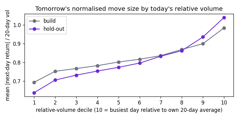
The decile picture is monotonic: the busiest tenth of stock-days, relative to their own history, are followed by moves about 60% larger than the quietest tenth.
5. Does volume add anything, holding today’s move fixed?
Within each date, regress the rank of the target on the ranks of both the baseline and the signal, and collect the slopes. This is the Fama–MacBeth construction on ranks; see beyond a baseline.
def per_date_slopes(d, cols, tgt="target"):
    def one(x):
        y = x[tgt].rank().values
        X = np.column_stack([np.ones(len(y))] + [x[c].rank().values for c in cols])
        return pd.Series(np.linalg.lstsq(X, y, rcond=None)[0][1:], index=cols)
    return d.groupby("date")[cols + [tgt]].apply(one)

slopes = per_date_slopes(test, ["base", "relvol"])
for c in slopes.columns:
    s = slopes[c]
    print("check   slope on rank(%s): mean %+.4f   t = %+.2f   days = %d" % (c, s.mean(), s.mean() / (s.std() / np.sqrt(len(s))), len(s)))
check slope on rank(base): mean +0.0442 t = +11.30 days = 399
check slope on rank(relvol): mean +0.0862 t = +24.69 days = 399Holding today’s move fixed, relative volume keeps a slope with a t of 25 on the hold-out. The boring explanation accounts for some of the pattern and not most of it.
6. Attack the result
Stability
ic = daily_ic(test, "relvol")
mid = test["date"].iloc[len(test) // 2]
report(ic[ic.index <= mid], "check, 1st half")
report(ic[ic.index > mid], "check, 2nd half")
ic_all = daily_ic(df, "relvol")
by_year = ic_all.groupby(ic_all.index.year).agg(["mean", "std", "count"])
by_year["t"] = by_year["mean"] / (by_year["std"] / np.sqrt(by_year["count"]))
print(by_year.round(4).to_string())
check, 1st half mean IC +0.1055 t = +22.03 hit = 0.94 days = 200
check, 2nd half mean IC +0.0964 t = +19.57 hit = 0.93 days = 199
mean std count t
date
2013 0.0707 0.0666 206 15.2162
2014 0.0811 0.0714 252 18.0312
2015 0.0863 0.0759 252 18.0662
2016 0.0830 0.0725 252 18.1911
2017 0.1029 0.0688 251 23.7062
2018 0.0782 0.0754 25 5.1803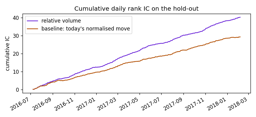
Show the code for this figure
import matplotlib.pyplot as plt

ic_base = daily_ic(test, "base")
fig, ax = plt.subplots(figsize=(7, 3.2))
ic.cumsum().plot(ax=ax, label="relative volume", color="#6d28d9")
ic_base.cumsum().plot(ax=ax, label="baseline: today's normalised move", color="#b45309")
ax.set_title("Cumulative daily rank IC on the hold-out")
ax.set_ylabel("cumulative IC")
ax.set_xlabel("")
ax.legend()
fig.tight_layout()
fig.savefig("relvol-cum-ic.png", dpi=120)
plt.show()
Both halves of the hold-out, every calendar year, and the cumulative-IC line is close to straight. This is what a stable relationship looks like; compare the reversal study, where the line climbed and went flat.
Sensitivity and horizon
extreme = df.loc[df["ret"].abs() > 0.25, ["date", "ticker"]]
kept = test.merge(extreme.assign(_x=1), on=["date", "ticker"], how="left")
report(daily_ic(kept[kept["_x"].isna()], "relvol"), "check, extremes removed")

for h in (1, 2, 5, 10, 20):
    col = "size%d" % h
    df[col] = df.groupby("ticker")["ret"].shift(-h).abs() / df["vol20"]
    d = df[df["date"] > cut + embargo].dropna(subset=[col])
    report(daily_ic(d, "relvol", col), "relvol vs move on day t+%d" % h)
check, extremes removed mean IC +0.1010 t = +29.36 hit = 0.93 days = 399
relvol vs move on day t+1 mean IC +0.1011 t = +29.36 hit = 0.93 days = 398
relvol vs move on day t+2 mean IC +0.0631 t = +20.56 hit = 0.85 days = 397
relvol vs move on day t+5 mean IC +0.0307 t = +9.65 hit = 0.68 days = 394
relvol vs move on day t+10 mean IC +0.0226 t = +7.07 hit = 0.66 days = 389
relvol vs move on day t+20 mean IC +0.0207 t = +6.59 hit = 0.64 days = 379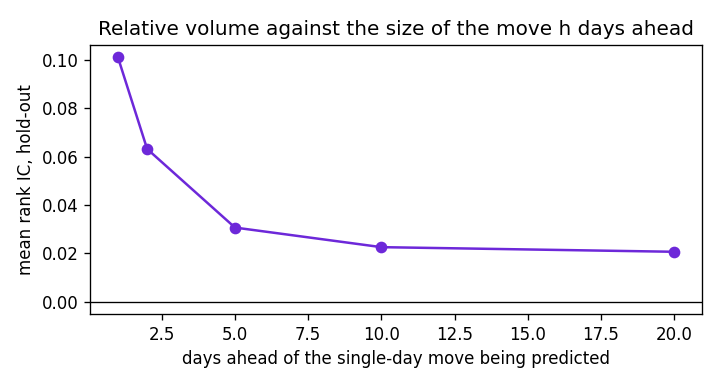
Show the code for this figure
import matplotlib.pyplot as plt

hs = (1, 2, 5, 10, 20)
hz = [daily_ic(df[df["date"] > cut + embargo].dropna(subset=["size%d" % h]), "relvol", "size%d" % h).mean() for h in hs]
fig, ax = plt.subplots(figsize=(6, 3.2))
ax.plot(hs, hz, marker="o", color="#6d28d9")
ax.axhline(0, color="k", lw=0.8)
ax.set_xlabel("days ahead of the single-day move being predicted")
ax.set_ylabel("mean rank IC, hold-out")
ax.set_title("Relative volume against the size of the move h days ahead")
fig.tight_layout()
fig.savefig("relvol-horizon-case.png", dpi=120)
plt.show()
Unchanged without the extreme rows. The information halves by day two and is still clearly there at day twenty: volatility information is slow, unlike direction information. See feature decay across horizons.
7. What the result means, and what it does not
An IC of 0.10 with a t of 29 is seven times the reversal study’s IC and looks spectacular next to it. It is not a trading signal in the same sense. The target is the size of a move, not its direction; knowing tomorrow will be a big day for a stock tells you nothing about which way. Sizes are far more predictable than signs, which is why every volatility model works and most return models do not.
What it is useful for: sizing positions, pricing short-dated options, deciding which names to watch. What it is not: evidence that volume predicts returns. The reversal study found that relative volume has no rank correlation with tomorrow’s signed return out of sample (see the model ladder).
The honest summary: relative volume predicts tomorrow’s normalised move size with an IC of about 0.10 out of sample, stable across years; about a third of that pattern is volatility clustering, and the rest survives controlling for it.
Slides
| # | Title | The sentence |
|---|---|---|
| 1 | The question as I read it | Cross-sectional; tomorrow’s move size in units of the stock’s own vol; predicted by today’s volume in units of the stock’s own average. |
| 2 | The data, and three things wrong with it | Same file and decisions as before; both quantities are heavy-tailed ratios, so ranks throughout. |
| 3 | How I decided what counts | Same split and embargo; the baseline is today’s move size, scored under identical rules. |
| 4 | Signal against baseline | Hold-out IC 0.10 for volume, 0.07 for today’s move, 0.106 for both. |
| 5 | Does it add anything | Per-date rank regression on both: volume keeps t = 25 holding today’s move fixed. |
| 6 | Does it hold | Both halves, every year; unchanged without extremes; half-life about two days, still positive at twenty. |
| 7 | What I’d do with another day | Test volume surprise (relative to the day of the week); split by market-wide volume days; check whether it adds to a GARCH-style vol forecast. |