The last three slides

Slides 5 to 7 of a seven-slide presentation, as a template. It is how every analysis ends.

Slide 5: what else I tried. One table, every signal that was scored, no exceptions, then one line.

signal	IC build	IC hold-out	t hold-out	days
(each thing you tried, simplest first)

Line under the table: “I tried N things. X held on the hold-out; Y and Z did not.”

Slide 6: does it hold. One sentence, one figure, one uncertainty line.

• Sentence: where in time the effect lives (first half / second half / every year / one year).
• Figure: the cumulative daily IC line (recipe below).
• Uncertainty line: “t of __ over __ days, having tried N things”, or the break-even cost if the study went as far as trading.

Slide 7: what I would do next. Always the same three questions, one line each.

1. Could it be fake? (the boring explanation not yet ruled out, and the test for it)
2. Can you trade it? (turnover, cost, capacity, or “not assessed”)
3. What would I run next, and why that first?

The code

Every figure ends the same way: save the PNG for the slide, then plt.show() so it also appears in the notebook. Shown here on one-day reversal in the equity file.

import pandas as pd, numpy as np
import matplotlib.pyplot as plt          # NOT matplotlib.use("Agg"): that line kills display in Jupyter

df = pd.read_csv("all_stocks_5yr.csv")
df["date"] = pd.to_datetime(df["date"])
df = df.rename(columns={"Name": "ticker"}).sort_values(["ticker", "date"]).reset_index(drop=True)
per = df.groupby("ticker").size()
df = df[df["ticker"].isin(per[per >= 1000].index)].copy()
g = df.groupby("ticker")
df["ret"] = g["close"].pct_change()
df["fwd_ret"] = g["ret"].shift(-1)
df["signal"] = -df["ret"]                # <- the SIGNAL column goes on the x-axis / into the IC, never the baseline
df = df.dropna(subset=["ret", "fwd_ret"])
cut, embargo = pd.Timestamp("2016-06-30"), pd.Timedelta(days=7)
test = df[df["date"] > cut + embargo].copy()

def daily_ic(d, sig, tgt="fwd_ret"):
    return d.groupby("date")[[sig, tgt]].apply(lambda x: x[sig].corr(x[tgt], method="spearman")).dropna()

# ---- Figure 1: cumulative daily IC line (slide 6) ----
ic = daily_ic(test, "signal")
fig, ax = plt.subplots(figsize=(8, 3.2))
ic.cumsum().plot(ax=ax)
ax.axhline(0, color="k", lw=0.8)
ax.set_title("Cumulative daily rank IC, hold-out  (mean %+.4f, t %+.2f, %d days)" % (ic.mean(), ic.mean() / (ic.std() / np.sqrt(len(ic))), len(ic)))
ax.set_ylabel("cumulative IC"); ax.set_xlabel("")
fig.tight_layout()
fig.savefig("fig_cum_ic.png", dpi=120)    # 1. save first, for PowerPoint
plt.show()                                # 2. then show, so it appears in the notebook
                                          # 3. no plt.close() here; only inside loops that make many figures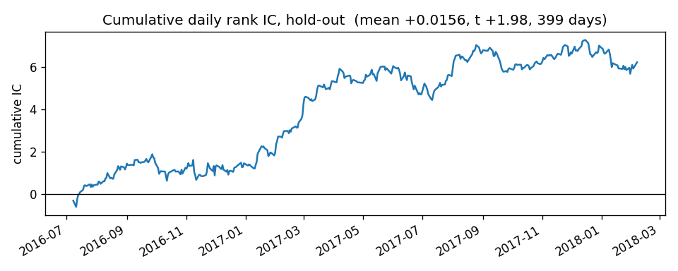

# ---- Figure 2: decile bar chart (slide 4 or 6) ----
test["dec"] = test.groupby("date")["signal"].transform(lambda x: pd.qcut(x.rank(method="first"), 10, labels=False))
dec = test.groupby("dec")["fwd_ret"].mean() * 1e4
fig, ax = plt.subplots(figsize=(6, 3.2))
ax.bar(dec.index + 1, dec.values)
ax.axhline(0, color="k", lw=0.8)
ax.set_xlabel("signal decile (1 = lowest, 10 = highest)"); ax.set_ylabel("mean next-day return, bps")
ax.set_title("Mean target by signal decile, hold-out")
fig.tight_layout()
fig.savefig("fig_deciles.png", dpi=120)
plt.show()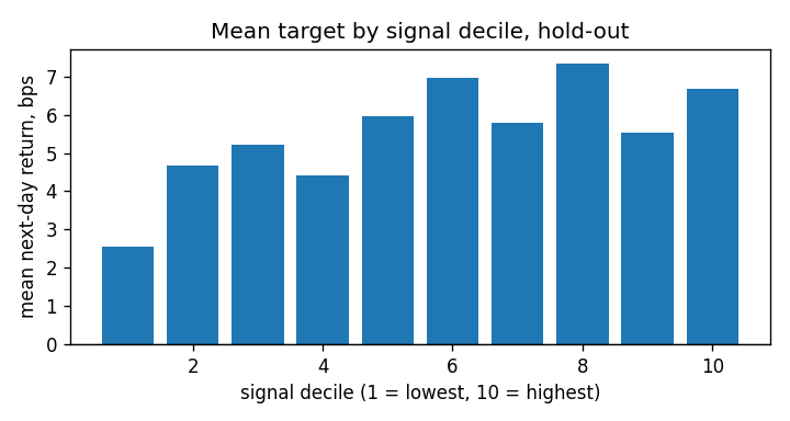

For the slide 5 table, add one (name, column) pair per signal scored, simplest first.

# ---- Slide 5 table: every signal scored ----
rows = []
train = df[df["date"] <= cut]
for name, col in (("1-day reversal", "signal"),):
    tr, te = daily_ic(train, col), daily_ic(test, col)
    rows.append({"signal": name, "IC build": tr.mean(), "IC hold-out": te.mean(),
                 "t hold-out": te.mean() / (te.std() / np.sqrt(len(te))), "days": len(te)})
print(pd.DataFrame(rows).round(4).to_string(index=False))

        signal  IC build  IC hold-out  t hold-out  days
1-day reversal    0.0114       0.0156      1.9781   399

Four more figures, each for one question (is it stable, does it survive, is it big, what does the input look like), continue from this code on charts as PNGs for slides.