
Hourly bike rentals: the random split that looked great
Two years of hourly rental counts with calendar and weather columns. A random split scores an R² of 0.86; training on the first year and testing on the second scores 0.63. Why the gap exists (the system grew), why adding a year column cannot fix it, and what does.
The most common way to get a wonderful number on time-stamped data is train_test_split with the default shuffle. This study measures exactly how wonderful, on a public table where the honest number is much lower, and then looks at why. The reason is not exotic. The thing being predicted grew over time, and a random split lets the model see the future level of the series while it is being tested on it.
The data: hourly rental counts from a city bike-share system for 2011 and 2012 (bike_hour.csv, from the UCI repository), with the calendar (hour, weekday, working day, holiday, month), the weather situation and normalised temperature, humidity and wind speed for each hour, and the count of rentals split into casual and registered users.
The question, as it arrived: “Predict the number of rentals in an hour from the calendar and the weather.”
1. Understand the data
import pandas as pd, numpy as np

df = pd.read_csv("bike_hour.csv")
df["t"] = pd.to_datetime(df["dteday"]) + pd.to_timedelta(df["hr"], unit="h")
df = df.sort_values("t").reset_index(drop=True)
print(df.shape, "|", df["t"].min(), "->", df["t"].max())
full = pd.date_range(df["t"].min(), df["t"].max(), freq="H")
print("hours in range: %d | rows: %d | missing hours: %d | nulls: %d | duplicate hours: %d"
      % (len(full), len(df), len(full) - len(df), int(df.isna().sum().sum()), df["t"].duplicated().sum()))
print("cnt == casual + registered on every row:", bool((df["cnt"] == df["casual"] + df["registered"]).all()))
print(df["cnt"].describe().round(0).to_string())
half = (df["t"].dt.month > 6).map({False: "H1", True: "H2"})
print("mean rentals per hour by half-year:", df.groupby([df["t"].dt.year, half])["cnt"].mean().round(0).to_dict())
(17379, 18) | 2011-01-01 00:00:00 -> 2012-12-31 23:00:00
hours in range: 17544 | rows: 17379 | missing hours: 165 | nulls: 0 | duplicate hours: 0
cnt == casual + registered on every row: True
count 17379.0
mean 189.0
std 181.0
min 1.0
25% 40.0
50% 142.0
75% 281.0
max 977.0
mean rentals per hour by half-year: {(2011, 'H1'): 123.0, (2011, 'H2'): 163.0, (2012, 'H1'): 215.0, (2012, 'H2'): 254.0}One row is one hour. The axis is nearly complete (165 hours missing out of 17,544, presumably hours with no rentals or no record). The target is a count: skewed, median 142, a long tail to 977. Two columns, casual and registered, add up to the target exactly and are excluded from every feature set below; they are the column that contains the answer in another costume.
The last line is the one that decides this study. Mean hourly rentals go from 123 in the first half of 2011 to 254 in the second half of 2012. The system doubled. Nothing in the calendar or weather columns says which year it is, except yr, which we come to.
2. The prediction boundary
Hour, weekday, holiday and month are known in advance. The weather columns are the weather that hour, which a real forecast would know only approximately; using them as given is an upper bound on what a live model could do, and is stated as such. The counts from previous hours are known if the forecast is made an hour ahead and not if it is made a week ahead, which is why the lag features appear only in section 7 with the horizon named. See prediction boundaries.
3. Three splits
feats = ["hr", "weekday", "workingday", "holiday", "mnth", "weathersit", "temp", "atemp", "hum", "windspeed"]
rng = np.random.RandomState(0)
shuffled = rng.permutation(len(df))
n_train = int(0.75 * len(df))
splits = {
    "random 75/25": (shuffled[:n_train], shuffled[n_train:]),
    "train 2011, test 2012": (np.where(df["yr"] == 0)[0], np.where(df["yr"] == 1)[0]),
    "train to Jun 2012, test Jul-Dec 2012": (np.where(df["t"] < "2012-07-01")[0], np.where(df["t"] >= "2012-07-01")[0]),
}
for name, (tr, te) in splits.items():
    print("%-38s train %5d rows (mean cnt %3.0f) | test %5d rows (mean cnt %3.0f)" % (name, len(tr), df["cnt"].iloc[tr].mean(), len(te), df["cnt"].iloc[te].mean()))
random 75/25 train 13034 rows (mean cnt 190) | test 4345 rows (mean cnt 187)
train 2011, test 2012 train 8645 rows (mean cnt 144) | test 8734 rows (mean cnt 235)
train to Jun 2012, test Jul-Dec 2012 train 13003 rows (mean cnt 168) | test 4376 rows (mean cnt 254)Under the random split the train and test sets have the same mean, because they are the same distribution. Under either chronological split the test period is busier than anything the model was trained on.
4. Baseline
The simplest thing that respects the shape of the data: the mean count for each (hour, working-day) cell, computed on the training rows.
def r2(y, yhat):
    return 1 - np.sum((y - yhat) ** 2) / np.sum((y - y.mean()) ** 2)

def mae(y, yhat):
    return np.mean(np.abs(y - yhat))

def score(name, label, pred, te):
    y = df["cnt"].values[te]
    print("%-38s %-42s R2 %+.3f  MAE %5.1f" % (name, label, r2(y, pred), mae(y, pred)))

def lookup_baseline(tr, te):
    table = df.iloc[tr].groupby(["hr", "workingday"])["cnt"].mean()
    keys = list(zip(df["hr"].iloc[te], df["workingday"].iloc[te]))
    return table.reindex(keys).values

for name, (tr, te) in splits.items():
    score(name, "baseline: train mean by hour x workingday", lookup_baseline(tr, te), te)
random 75/25 baseline: train mean by hour x workingday R2 +0.625 MAE 72.4
train 2011, test 2012 baseline: train mean by hour x workingday R2 +0.435 MAE 108.5
train to Jun 2012, test Jul-Dec 2012 baseline: train mean by hour x workingday R2 +0.532 MAE 107.2A 48-cell lookup table explains 63% of the variance under a random split and 44% of it a year ahead. Everything below has to be read against these numbers.
5. The model, and the number that lies
A random forest on the ten calendar and weather columns, then the same forest with the yr column added.
from sklearn.ensemble import RandomForestRegressor

def forest(tr, te, cols):
    m = RandomForestRegressor(n_estimators=100, min_samples_leaf=3, random_state=0, n_jobs=-1)
    return m.fit(df[cols].values[tr], df["cnt"].values[tr]).predict(df[cols].values[te])

for name, (tr, te) in splits.items():
    score(name, "forest: calendar + weather", forest(tr, te, feats), te)
    score(name, "forest: calendar + weather + year", forest(tr, te, feats + ["yr"]), te)
random 75/25 forest: calendar + weather R2 +0.858 MAE 44.5
random 75/25 forest: calendar + weather + year R2 +0.938 MAE 26.3
train 2011, test 2012 forest: calendar + weather R2 +0.633 MAE 90.0
train 2011, test 2012 forest: calendar + weather + year R2 +0.633 MAE 90.0
train to Jun 2012, test Jul-Dec 2012 forest: calendar + weather R2 +0.651 MAE 92.5
train to Jun 2012, test Jul-Dec 2012 forest: calendar + weather + year R2 +0.891 MAE 47.0Same model, same columns: R² 0.86 when rows are shuffled, 0.63 when 2011 predicts 2012. The mean absolute error doubles. Adding yr pushes the random-split number to 0.94 and does nothing for the year-ahead number, because a tree trained on rows where yr is always 0 has never seen a 1 and treats it as a 0. A column that takes a new value in the test period cannot help a tree; it is a label for the future, not a feature.
The third split is the fair version of what a model in use would face: trained on eighteen months, asked about the next six. It is only slightly better than the year-ahead split, and adding yr now helps, because the training set contains six months of 2012 to learn its level from.
6. Why: the residuals have a sign
tr, te = splits["train 2011, test 2012"]
pred = forest(tr, te, feats)
resid = pd.Series(df["cnt"].values[te] - pred, index=df["t"].iloc[te])
print("mean residual (actual - predicted) by quarter of 2012:")
print(resid.groupby(resid.index.quarter).agg(["mean", "count"]).round(1).to_string())
print("mean of the model's predictions %.0f | mean actual %.0f" % (pred.mean(), df["cnt"].values[te].mean()))
mean residual (actual - predicted) by quarter of 2012:
mean count
t
1 79.9 2176
2 83.5 2182
3 97.5 2208
4 75.4 2168
mean of the model's predictions 151 | mean actual 235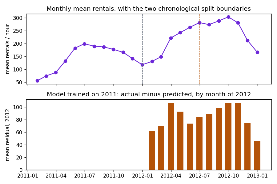
Show the code for this figure
import matplotlib.pyplot as plt

monthly = df.set_index("t")["cnt"].resample("M").mean()
fig, (a1, a2) = plt.subplots(2, 1, figsize=(7.5, 5), sharex=True)
a1.plot(monthly.index, monthly.values, marker="o", color="#6d28d9")
a1.axvline(pd.Timestamp("2012-01-01"), color="#6b7280", ls="--", lw=0.9)
a1.axvline(pd.Timestamp("2012-07-01"), color="#b45309", ls="--", lw=0.9)
a1.set_ylabel("mean rentals / hour")
a1.set_title("Monthly mean rentals, with the two chronological split boundaries")
rm = resid.resample("M").mean()
a2.bar(rm.index, rm.values, width=20, color="#b45309")
a2.axhline(0, color="k", lw=0.8)
a2.set_ylabel("mean residual, 2012")
a2.set_title("Model trained on 2011: actual minus predicted, by month of 2012")
fig.tight_layout()
fig.savefig("bike-growth-and-residuals.png", dpi=120)
plt.show()
The model trained on 2011 predicts a 2011-sized city. In every quarter of 2012 the actual count exceeds the prediction by 75 to 98 rentals an hour on average. A random split never shows this, because three-quarters of every month of 2012 is in the training set: the forest learns the December 2012 level from December 2012 rows and is then tested on the remaining December 2012 rows. That is the leak. It is not a wrong shift or a stray column; it is the split itself letting the model see the level of the series at the time it is being tested on.
7. What fixes it: features that carry the level
If the forecast is made a day or an hour ahead, recent counts are known, and they carry the current level of the series in a way no calendar column can. The lags are built only where the previous row really is the previous hour, so the 165 missing hours cannot produce a wrong lag.
gap = df["t"].diff().dt.total_seconds() / 3600
df["lag1"] = df["cnt"].shift(1).where(gap == 1)                                                 # the previous hour, when it exists
df["lag24"] = df["cnt"].shift(24).where(df["t"] - df["t"].shift(24) == pd.Timedelta(hours=24))   # same hour yesterday
df["lag168"] = df["cnt"].shift(168).where(df["t"] - df["t"].shift(168) == pd.Timedelta(hours=168))   # same hour last week
ok = df[["lag1", "lag24", "lag168"]].notna().all(axis=1).values
name = "train to Jun 2012, test Jul-Dec 2012"
tr, te = splits[name]
tr, te = tr[ok[tr]], te[ok[te]]
score(name, "naive: same hour last week (lag168)", df["lag168"].values[te], te)
score(name, "forest: calendar + weather", forest(tr, te, feats), te)
score(name, "forest: + lag24 + lag168  (day-ahead)", forest(tr, te, feats + ["lag24", "lag168"]), te)
score(name, "forest: + lag1 + lag24 + lag168  (hour-ahead)", forest(tr, te, feats + ["lag1", "lag24", "lag168"]), te)
train to Jun 2012, test Jul-Dec 2012 naive: same hour last week (lag168) R2 +0.798 MAE 58.6
train to Jun 2012, test Jul-Dec 2012 forest: calendar + weather R2 +0.645 MAE 95.4
train to Jun 2012, test Jul-Dec 2012 forest: + lag24 + lag168 (day-ahead) R2 +0.871 MAE 49.1
train to Jun 2012, test Jul-Dec 2012 forest: + lag1 + lag24 + lag168 (hour-ahead) R2 +0.926 MAE 37.9Three things to read off. The naive forecast is strong: “same as this hour last week” explains 80% of the variance on its own, more than the calendar-and-weather forest. The lags fix the level problem: with last week’s and yesterday’s counts the forest is at 0.87 a day ahead, and with the previous hour it is at 0.93 an hour ahead. The horizon decides the feature set: lag1 is only available to an hour-ahead forecast, and a page that reports 0.93 without saying “one hour ahead” is reporting a number for a different problem. See feature decay across horizons.
8. One more thing the table shows: an interaction
The hour-of-day pattern is not one curve; it is two, depending on whether people are commuting.
pv = df.pivot_table(index="workingday", columns="hr", values="cnt", aggfunc="mean").round(0)
print(pv[[6, 8, 10, 12, 14, 17, 19, 22]].to_string())
hr 6 8 10 12 14 17 19 22
workingday
0 19.0 106.0 256.0 366.0 365.0 324.0 232.0 116.0
1 102.0 477.0 135.0 201.0 184.0 525.0 348.0 138.0Working days peak at 8 and 17; non-working days peak at 13. A model that treats hour and working-day as separate additive effects cannot represent that, and the difference is measurable:
from sklearn.linear_model import Ridge

tr, te = splits["train to Jun 2012, test Jul-Dec 2012"]
weather = df[["temp", "hum", "windspeed"]]
additive = pd.concat([pd.get_dummies(df[["hr", "workingday"]].astype(str), dtype=float), weather], axis=1)
pair = (df["hr"].astype(str) + "_" + df["workingday"].astype(str)).rename("hr_wd")
interact = pd.concat([pd.get_dummies(pair, dtype=float), weather], axis=1)

def ridge_r2(X):
    m = Ridge(alpha=1.0).fit(X.values[tr], np.log1p(df["cnt"].values[tr]))
    return r2(df["cnt"].values[te], np.expm1(m.predict(X.values[te])))

print("ridge on log(1 + cnt): hour and workingday as separate dummies   R2 %.3f" % ridge_r2(additive))
print("ridge on log(1 + cnt): one dummy per (hour, workingday) pair      R2 %.3f" % ridge_r2(interact))
ridge on log(1 + cnt): hour and workingday as separate dummies R2 0.403
ridge on log(1 + cnt): one dummy per (hour, workingday) pair R2 0.600Same linear model, same information, one interaction term: R² 0.40 to 0.60 on the same chronological test. The forest finds this interaction on its own, which is most of what it is adding over the lookup baseline. When a linear model underperforms a tree by a wide margin on a small feature set, the first suspect is an interaction like this one, not a missing feature. See choosing a model.
9. What to say
Under a random split a forest on calendar and weather explains 86% of the hourly variance; trained on 2011 and tested on 2012 it explains 63%, because rentals doubled over the two years and a shuffled split lets the model learn each month’s level from that month’s own rows. Adding a year column does not help a year ahead. What helps is giving the model recent counts: with last week’s and yesterday’s values it reaches 0.87 a day ahead, against 0.80 for simply repeating last week’s value. The weather columns are the actual weather, so all of this is an upper bound on what a forecast-driven model could do.
Takeaways
- On time-stamped data, a shuffled split is a leak whenever the level of the series moves. The leak is invisible in the score and obvious in a plot of the monthly mean.
- A feature that takes unseen values in the test period (a year indicator, a row index, a date as a number) cannot help a tree and will not help a linear model in a way that generalises.
- The seasonal naive forecast is the baseline, not the mean. Here it beats a ten-feature forest.
- Name the horizon. The feature set depends on it; the score means nothing without it.
- Look at residuals by time. A model that is wrong in the same direction for twelve months in a row is not noisy; it is missing a level.
For a series where the same comparison comes out the other way, because nothing drifts, see hourly traffic volume against a seasonal baseline. For the general rule, choosing a train/test split; for the equity version of the same leak, chronological splits with an embargo.