
Twelve monitoring sites, one sky: a panel where the entity does not matter
Four years of hourly air-quality readings at twelve sites, aggregated to station-days, with tomorrow's PM2.5 as the target. Holding out whole stations changes nothing; holding out dates cuts the forest's R² from 0.72 to 0.35. Which axis of a panel carries the variance decides which split is honest, and here it is the opposite of the patient data.
A panel has two axes, entities and time, and either can carry the correlation that makes a random split lie. The Parkinson’s study is the case where the entity carries almost all of it: 93% of the target’s variance was which subject. This is the other case. Twelve monitoring sites in one city breathe the same air, so the date carries almost everything and the site almost nothing, and the split that matters is by time.
The data: hourly readings of six pollutants and five weather variables at twelve air-quality monitoring sites from March 2013 to February 2017 (beijing_air_quality.csv, UCI repository, Zhang et al. 2017; the twelve per-site files are concatenated). The study works at the station-day level.
The question, as it arrived: “Predict tomorrow’s PM2.5 at each site from today’s readings.”
1. Understand the data
import pandas as pd, numpy as np

hourly = pd.read_csv("beijing_air_quality.csv")
hourly["date"] = pd.to_datetime(hourly[["year", "month", "day"]])
print(hourly.shape, "| stations:", hourly["station"].nunique(), "| hours per station:", hourly.groupby("station").size().unique().tolist())
print("null share:", hourly[["PM2.5", "PM10", "SO2", "NO2", "CO", "O3", "TEMP", "WSPM"]].isna().mean().round(3).to_dict())
pol = ["PM2.5", "PM10", "SO2", "NO2", "CO", "O3"]
met = ["TEMP", "PRES", "DEWP", "RAIN", "WSPM"]
d = hourly.groupby(["station", "date"])[pol + met].mean().reset_index().sort_values(["station", "date"]).reset_index(drop=True)
print("station-days:", len(d), "| daily PM2.5: median %.0f, mean %.0f, max %.0f, skew %.1f" % (d["PM2.5"].median(), d["PM2.5"].mean(), d["PM2.5"].max(), d["PM2.5"].skew()))
wide = d.pivot(index="date", columns="station", values="PM2.5")
c = wide.corr().values
print("same-day PM2.5 correlation between stations: mean %.2f, min %.2f" % (c[np.triu_indices(12, 1)].mean(), c[np.triu_indices(12, 1)].min()))
print("mean daily PM2.5 by station:", d.groupby("station")["PM2.5"].mean().round(0).astype(int).to_dict())
(420768, 19) | stations: 12 | hours per station: [35064]
null share: {'PM2.5': 0.021, 'PM10': 0.015, 'SO2': 0.021, 'NO2': 0.029, 'CO': 0.049, 'O3': 0.032, 'TEMP': 0.001, 'WSPM': 0.001}
station-days: 17532 | daily PM2.5: median 60, mean 80, max 567, skew 1.9
same-day PM2.5 correlation between stations: mean 0.95, min 0.87
mean daily PM2.5 by station: {'Aotizhongxin': 83, 'Changping': 71, 'Dingling': 66, 'Dongsi': 86, 'Guanyuan': 83, 'Gucheng': 84, 'Huairou': 70, 'Nongzhanguan': 85, 'Shunyi': 80, 'Tiantan': 82, 'Wanliu': 83, 'Wanshouxigong': 85}One row, after aggregation, is one station on one day. A complete grid of twelve stations by 1,461 days, with a few percent of hourly readings missing. The target is right-skewed (mean above median, skew 2), so the models below fit log(1 + PM2.5) and are scored on the original scale. And the number that decides the study: the daily PM2.5 series of any two stations correlate at about 0.95. Station means differ by about 30%; day-to-day swings differ by a factor of ten.
2. Target, features and where the variance is
g = d.groupby("station")
d["y_next"] = g["PM2.5"].shift(-1)                                                  # target: tomorrow's daily mean, same station
d["pm_lag1"] = g["PM2.5"].shift(1)
d["pm_ma7"] = g["PM2.5"].transform(lambda s: s.rolling(7, min_periods=3).mean())   # ends today, which is known
doy = d["date"].dt.dayofyear
d["doy_sin"], d["doy_cos"] = np.sin(2 * np.pi * doy / 365.25), np.cos(2 * np.pi * doy / 365.25)
d["dow"], d["month"] = d["date"].dt.dayofweek, d["date"].dt.month
feats = pol + met + ["pm_lag1", "pm_ma7", "doy_sin", "doy_cos", "dow"]
dd = d.dropna(subset=feats + ["y_next"]).reset_index(drop=True)
dd["log_y"] = np.log1p(dd["y_next"])
print("usable station-days: %d | %s -> %s" % (len(dd), dd["date"].min().date(), dd["date"].max().date()))
by_station = dd.groupby("station")["log_y"].transform("mean")
by_date = dd.groupby("date")["log_y"].transform("mean")
print("variance of log(1 + tomorrow's PM2.5): %.3f | share explained by which station: %.1f%% | by which date: %.1f%%"
      % (dd["log_y"].var(), 100 * by_station.var() / dd["log_y"].var(), 100 * by_date.var() / dd["log_y"].var()))
print("correlation of today's and tomorrow's daily PM2.5 at a station: %.2f" % dd["PM2.5"].corr(dd["y_next"]))
usable station-days: 16880 | 2013-03-03 -> 2017-02-27
variance of log(1 + tomorrow's PM2.5): 0.774 | share explained by which station: 1.4% | by which date: 94.4%
correlation of today's and tomorrow's daily PM2.5 at a station: 0.57Which station explains 1.4% of the variance. Which date explains 94%. Everything in this table is about days, not places. And tomorrow correlates with today at only 0.57, so day-ahead pollution is genuinely hard to forecast; the baselines will be weak and the honest model will not be much better.
3. Four validation designs
The same rows, the same features, four ways of deciding what is train and what is test.
cut = pd.Timestamp("2016-03-01")
held = ["Huairou", "Wanshouxigong", "Guanyuan"]                        # three of the twelve, chosen once at random
rng = np.random.RandomState(0)
idx = rng.permutation(len(dd))
n = int(0.75 * len(dd))
is_held = dd["station"].isin(held).values
later = (dd["date"] >= cut).values
designs = {
    "random rows": (idx[:n], idx[n:]),
    "chronological": (np.where(~later)[0], np.where(later)[0]),
    "stations held out, all dates": (np.where(~is_held)[0], np.where(is_held)[0]),
    "stations held out, later dates": (np.where(~is_held & ~later)[0], np.where(is_held & later)[0]),
}
for name, (tr, te) in designs.items():
    shared_dates = dd["date"].iloc[te].isin(dd["date"].iloc[tr]).mean()
    shared_stations = len(set(dd["station"].iloc[te]) & set(dd["station"].iloc[tr]))
    print("%-32s train %5d  test %4d | share of test dates also in train: %.2f | test stations also in train: %d" % (name, len(tr), len(te), shared_dates, shared_stations))
random rows train 12660 test 4220 | share of test dates also in train: 1.00 | test stations also in train: 12
chronological train 12579 test 4301 | share of test dates also in train: 0.00 | test stations also in train: 12
stations held out, all dates train 12591 test 4289 | share of test dates also in train: 1.00 | test stations also in train: 0
stations held out, later dates train 9371 test 1081 | share of test dates also in train: 0.00 | test stations also in train: 0Under the random split, every test row’s date is in the training set, eleven times over. Under the station hold-out with all dates, the same is true. Only the two chronological designs put the test dates outside the training data.
4. Baselines and models under each design
from sklearn.linear_model import Ridge
from sklearn.ensemble import RandomForestRegressor

def r2(y, yhat):
    return 1 - np.sum((y - yhat) ** 2) / np.sum((y - y.mean()) ** 2)

def mae(y, yhat):
    return np.mean(np.abs(y - yhat))

results = {}
def score(design, label, pred, te):
    y = dd["y_next"].values[te]
    results[(design, label)] = r2(y, pred)
    print("%-32s %-36s R2 %+.3f  MAE %5.1f" % (design, label, r2(y, pred), mae(y, pred)))

X = dd[feats].values
for design, (tr, te) in designs.items():
    score(design, "baseline: persistence (today's value)", dd["PM2.5"].values[te], te)
    clim = dd.iloc[tr].groupby("month")["y_next"].mean()
    score(design, "baseline: train mean by month", dd["month"].iloc[te].map(clim).values, te)
    m = Ridge(alpha=1.0).fit(X[tr], dd["log_y"].values[tr])
    score(design, "ridge on log target", np.expm1(m.predict(X[te])), te)
    m = RandomForestRegressor(n_estimators=60, min_samples_leaf=5, random_state=0, n_jobs=-1).fit(X[tr], dd["log_y"].values[tr])
    score(design, "forest on log target", np.expm1(m.predict(X[te])), te)
random rows baseline: persistence (today's value) R2 +0.172 MAE 44.5
random rows baseline: train mean by month R2 +0.053 MAE 50.8
random rows ridge on log target R2 +0.349 MAE 38.4
random rows forest on log target R2 +0.724 MAE 23.1
chronological baseline: persistence (today's value) R2 +0.163 MAE 44.2
chronological baseline: train mean by month R2 +0.066 MAE 50.2
chronological ridge on log target R2 +0.291 MAE 39.0
chronological forest on log target R2 +0.367 MAE 36.7
stations held out, all dates baseline: persistence (today's value) R2 +0.151 MAE 43.7
stations held out, all dates baseline: train mean by month R2 +0.057 MAE 49.9
stations held out, all dates ridge on log target R2 +0.344 MAE 37.4
stations held out, all dates forest on log target R2 +0.747 MAE 20.4
stations held out, later dates baseline: persistence (today's value) R2 +0.188 MAE 43.7
stations held out, later dates baseline: train mean by month R2 +0.064 MAE 50.3
stations held out, later dates ridge on log target R2 +0.303 MAE 38.7
stations held out, later dates forest on log target R2 +0.351 MAE 36.8Read the forest row across the four designs. Random rows: about 0.72. Stations held out but dates shared: about 0.75, better than random, because the model has never seen these stations and does not care. Chronological: about 0.37. Stations held out and later dates: about 0.35, the same as chronological within noise. Holding out stations changes nothing; holding out time halves the score.
The ridge is worth reading too: it gains far less from the leak (0.35 to 0.29), because a linear model cannot memorise a date from a combination of pollutant readings the way a forest can. The leaky number is not “the forest is a better model”; it is “the forest is a better lookup table”.
5. Naming the leak
If the date is what leaks, holding out random dates (all twelve stations of each held-out day together) should give the chronological number even though the held-out days are scattered through the four years.
dates = np.sort(dd["date"].unique())
rng2 = np.random.RandomState(1)
held_dates = set(rng2.choice(dates, int(0.25 * len(dates)), replace=False))
te = np.where(dd["date"].isin(held_dates))[0]
tr = np.where(~dd["date"].isin(held_dates))[0]
m = RandomForestRegressor(n_estimators=60, min_samples_leaf=5, random_state=0, n_jobs=-1).fit(X[tr], dd["log_y"].values[tr])
score("random dates held out", "forest on log target", np.expm1(m.predict(X[te])), te)
score("random dates held out", "baseline: persistence (today's value)", dd["PM2.5"].values[te], te)
random dates held out forest on log target R2 +0.323 MAE 35.8
random dates held out baseline: persistence (today's value) R2 +0.123 MAE 40.4It does. Scattered dates with all their stations held out score close to the chronological split, and nowhere near the random-row number. The leak was never about the future; it was about the other eleven rows of the same day. Under a random row split the forest sees, for almost every test row, what happened tomorrow at eleven neighbouring sites, and since tomorrow’s PM2.5 is a regional event, that is most of the answer.
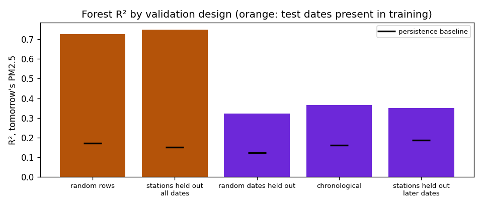
Show the code for this figure
import matplotlib.pyplot as plt

order = ["random rows", "stations held out, all dates", "random dates held out", "chronological", "stations held out, later dates"]
vals = [results[(k, "forest on log target")] for k in order]
base = [results[(k, "baseline: persistence (today's value)")] for k in order]
fig, ax = plt.subplots(figsize=(8, 3.4))
ax.bar(range(5), vals, color=["#b45309", "#b45309", "#6d28d9", "#6d28d9", "#6d28d9"])
ax.plot(range(5), base, "k_", ms=22, mew=2, label="persistence baseline")
ax.set_xticks(range(5))
ax.set_xticklabels([k.replace(", ", "\n") for k in order], fontsize=8)
ax.set_ylabel("R², tomorrow's PM2.5")
ax.set_title("Forest R² by validation design (orange: test dates present in training)")
ax.legend(fontsize=8)
fig.tight_layout()
fig.savefig("beijing-r2-by-design.png", dpi=120)
plt.show()
6. What to say
Tomorrow’s daily PM2.5 at a site can be predicted from today’s readings with an R² of about 0.37 on the final year, against 0.16 for assuming tomorrow equals today; the mean error is about 37 on a series whose daily median is 60. A random split reports 0.72, which is not a forecast: twelve sites share each day’s pollution almost exactly, so a shuffled split shows the model tomorrow’s value at eleven neighbours. Holding out whole sites does not fix it; holding out days does. The site identity explains 1% of the variance and can be ignored; the date explains 94% and must be split on.
Takeaways
- Decompose the target’s variance along every axis of the panel before choosing a split: by entity, by time, by whatever else groups the rows. The axis with the variance is the axis to hold out.
- “Grouped split” does not mean “split by the identifier column”. It means split by whatever the rows share. Here rows share a day.
- A forest gains far more from a leak than a linear model. When the gap between the two widens dramatically under one design and closes under another, suspect the design, not the model.
- Weak forecasts are still forecasts. An honest 0.37 against a persistence baseline of 0.16 is a result; a leaked 0.72 is not.
- Repeated entities are not always the problem. The Parkinson’s study is this table with the axes swapped; the check is the same, and the answer is the opposite.
For the general rule, see choosing a train/test split; for the equity version, where every stock shares each date’s market move, chronological splits with an embargo and single series or panel.