Hourly traffic volume: a messy clock and a baseline that is hard to beat

The bike-rental study showed a random split inflating a forecast’s score from 0.63 to 0.86 because the series grew. This is the control experiment: a series of the same kind, hourly counts with calendar and weather, on which the same comparison comes out even. The lesson is not that shuffled splits are safe. It is why they were safe here, and that the answer can be read off one line of output before any model is fitted. Before that, the table’s clock has to be repaired, which is most of the work.

The data: hourly westbound traffic volume on Interstate 94 between Minneapolis and St Paul, October 2012 to September 2018, with weather and a holiday column (metro_traffic.csv, UCI repository, Hogue 2019).

The question, as it arrived: “Forecast the hourly traffic volume.” As in the load-forecasting study, the horizon has to be named; the main comparison here is a day ahead, with one hour ahead shown for contrast.

1. Understand the data, starting with the clock

import pandas as pd, numpy as np

raw = pd.read_csv("metro_traffic.csv")
raw["t"] = pd.to_datetime(raw["date_time"])
print(raw.shape, "|", raw["t"].min(), "->", raw["t"].max())
print("exact duplicate rows: %d | duplicate timestamps: %d" % (raw.duplicated().sum(), raw["t"].duplicated().sum()))
same_t = raw[raw["t"].duplicated(keep=False)]
print("timestamps with several rows: %d; of these, rows disagree on traffic_volume in %d, on weather_description in %d"
      % (same_t["t"].nunique(), (same_t.groupby("t")["traffic_volume"].nunique() > 1).sum(), (same_t.groupby("t")["weather_description"].nunique() > 1).sum()))
print("holiday column: non-null in %d rows; values:" % raw["holiday"].notna().sum(), raw["holiday"].dropna().unique()[:4].tolist(), "...")
print(raw[["temp", "rain_1h", "snow_1h", "clouds_all", "traffic_volume"]].describe().loc[["min", "50%", "max"]].round(1).to_string())
print("rows with temp == 0 K: %d | rows with rain_1h > 100 mm: %d" % ((raw["temp"] == 0).sum(), (raw["rain_1h"] > 100).sum()))

(48204, 10) | 2012-10-02 09:00:00 -> 2018-09-30 23:00:00
exact duplicate rows: 17 | duplicate timestamps: 7629
timestamps with several rows: 5445; of these, rows disagree on traffic_volume in 0, on weather_description in 5386
holiday column: non-null in 61 rows; values: ['Columbus Day', 'Veterans Day', 'Thanksgiving Day', 'Christmas Day'] ...
      temp  rain_1h  snow_1h  clouds_all  traffic_volume
min    0.0      0.0      0.0         0.0             0.0
50%  282.4      0.0      0.0        64.0          3380.0
max  310.1   9831.3      0.5       100.0          7280.0
rows with temp == 0 K: 10 | rows with rain_1h > 100 mm: 1

One row is supposed to be one hour, and 7,629 of them are not: when the weather station reported two conditions for an hour (“mist” and “haze”), the traffic count was written out twice. The counts agree on every duplicated timestamp, so the duplicates carry no information and would double-count those hours in any score. The holiday column is null except on holidays, which is a sentinel for “no”, not a gap. Ten rows have a temperature of 0 kelvin and one has 9,831 mm of rain in an hour, which are recording failures, not weather. None of this is visible from df.describe() alone; the duplicate-timestamp check and the physical-range check are separate lines. See first-pass dataset interrogation.

d = raw.drop_duplicates("t").sort_values("t").reset_index(drop=True)        # one row per hour; the twins only disagreed on the weather text
d.loc[d["temp"] == 0, "temp"] = np.nan
d["temp"] = d["temp"].interpolate()
d.loc[d["rain_1h"] > 100, "rain_1h"] = 0.0
gap = d["t"].diff().dt.total_seconds() / 3600
print("rows after removing duplicate timestamps: %d | gaps longer than an hour: %d | longest gap: %.0f hours, starting %s" % (len(d), (gap > 1).sum(), gap.max(), d.loc[gap.idxmax() - 1, "t"]))
d["hour"], d["dow"], d["month"], d["year"] = d["t"].dt.hour, d["t"].dt.dayofweek, d["t"].dt.month, d["t"].dt.year
d["holiday_flag"] = d["holiday"].notna().astype(int)
print("rows per year:", d["year"].value_counts().sort_index().to_dict())
print("mean hourly volume by year:", d.groupby("year")["traffic_volume"].mean().round(0).astype(int).to_dict())

rows after removing duplicate timestamps: 40575 | gaps longer than an hour: 2588 | longest gap: 7387 hours, starting 2014-08-08 01:00:00
rows per year: {2012: 2103, 2013: 7294, 2014: 4501, 2015: 3593, 2016: 7838, 2017: 8713, 2018: 6533}
mean hourly volume by year: {2012: 3227, 2013: 3310, 2014: 3270, 2015: 3258, 2016: 3194, 2017: 3377, 2018: 3324}

After deduplication there are 40,575 hours out of the 52,000 the six years contain: 2,588 gaps, including one of ten months in 2014 and 2015. The gaps matter for lag features (the row 24 positions back is not always 24 hours back) and are handled below. The last line is the one that predicts the outcome of this study: the yearly means sit within 6% of each other, between about 3,190 and 3,380 vehicles an hour. Nothing grew.

2. Features and the prediction boundary

Calendar columns are known in advance. The weather columns are the weather at the hour, an upper bound for a day-ahead forecast, kept because they turn out not to matter. Lags are built only where the row that far back really is that many hours back.

def lag(hours):
    return d["traffic_volume"].shift(hours).where(d["t"] - d["t"].shift(hours) == pd.Timedelta(hours=hours))

d["lag1"], d["lag24"], d["lag168"] = lag(1), lag(24), lag(168)
print("share of rows with a valid lag: 1h %.2f | 24h %.2f | 168h %.2f" % (d["lag1"].notna().mean(), d["lag24"].notna().mean(), d["lag168"].notna().mean()))

share of rows with a valid lag: 1h 0.94 | 24h 0.71 | 168h 0.42

Only 42% of rows have a clean “same hour last week”, because a week has to contain no gap at either end. A lag computed by row position instead would silently pair hours across the ten-month hole.

3. Split, baselines, and the comparison the bike data failed

Chronological: train on 2012 to 2017, test on 2018. A shuffled 75/25 split is run alongside it for the one purpose of measuring the difference.

from sklearn.ensemble import RandomForestRegressor

def r2(y, yhat):
    return 1 - np.sum((y - yhat) ** 2) / np.sum((y - y.mean()) ** 2)

def mae(y, yhat):
    return np.mean(np.abs(y - yhat))

cal = ["hour", "dow", "month", "holiday_flag"]
weather = ["temp", "rain_1h", "snow_1h", "clouds_all"]

def forest(tr, te, cols):
    m = RandomForestRegressor(n_estimators=100, min_samples_leaf=3, random_state=0, n_jobs=-1)
    return m.fit(d[cols].values[tr], d["traffic_volume"].values[tr]).predict(d[cols].values[te])

def score(label, te, pred):
    y = d["traffic_volume"].values[te]
    print("%-58s R2 %.3f  MAE %4.0f vehicles/hour" % (label, r2(y, pred), mae(y, pred)))

rng = np.random.RandomState(0)
idx = rng.permutation(len(d))
n = int(0.75 * len(d))
random_tr, random_te = idx[:n], idx[n:]
chrono_tr, chrono_te = np.where(d["year"] <= 2017)[0], np.where(d["year"] == 2018)[0]
print("chronological: train 2012-2017 (%d hours), test 2018 (%d hours)" % (len(chrono_tr), len(chrono_te)))
table = d.iloc[chrono_tr].groupby(["hour", "dow"])["traffic_volume"].mean()
score("baseline: train mean by hour x weekday, 2018", chrono_te, table.reindex(list(zip(d["hour"].iloc[chrono_te], d["dow"].iloc[chrono_te]))).values)
for c in ("lag1", "lag24", "lag168"):
    ok = chrono_te[d[c].notna().values[chrono_te]]
    score("naive: %s, 2018 (%d hours where available)" % (c, len(ok)), ok, d[c].values[ok])
score("forest, calendar + weather: shuffled split", random_te, forest(random_tr, random_te, cal + weather))
score("forest, calendar + weather: 2018", chrono_te, forest(chrono_tr, chrono_te, cal + weather))
score("forest, calendar only: 2018", chrono_te, forest(chrono_tr, chrono_te, cal))

chronological: train 2012-2017 (34042 hours), test 2018 (6533 hours)
baseline: train mean by hour x weekday, 2018               R2 0.944  MAE  265 vehicles/hour
naive: lag1, 2018 (6521 hours where available)             R2 0.830  MAE  589 vehicles/hour
naive: lag24, 2018 (6247 hours where available)            R2 0.726  MAE  567 vehicles/hour
naive: lag168, 2018 (4933 hours where available)           R2 0.886  MAE  344 vehicles/hour
forest, calendar + weather: shuffled split                 R2 0.946  MAE  272 vehicles/hour
forest, calendar + weather: 2018                           R2 0.948  MAE  254 vehicles/hour
forest, calendar only: 2018                                R2 0.949  MAE  246 vehicles/hour

Three results. The hour-by-weekday lookup table already scores 0.94, because traffic is a schedule. The shuffled and chronological splits give the same number, 0.95 either way: the series has no trend, so the shuffled split has no future level to leak, and the score it reports is honest by accident. And weather adds nothing to the calendar; a null result, and a cheap one to keep.

Compare the bike data, where the same forest went from 0.86 shuffled to 0.63 chronological. The difference between the two tables is entirely in the “mean by year” line above. Check it before trusting either kind of split, and if it moves, the shuffled number is not a forecast.

4. Lags, on the rows where they exist

The naive forecasts and the lag features are only defined where the clock is intact, so the fair comparison restricts every model to the same rows.

have = d[["lag24", "lag168"]].notna().all(axis=1).values
tr, te = chrono_tr[have[chrono_tr]], chrono_te[have[chrono_te]]
print("day-ahead comparison on the %d hours of 2018 with clean 24h and 168h lags" % len(te))
score("naive: same hour last week", te, d["lag168"].values[te])
score("forest: calendar + weather", te, forest(tr, te, cal + weather))
score("forest: + lag24 + lag168", te, forest(tr, te, cal + weather + ["lag24", "lag168"]))
have1 = d["lag1"].notna().values
tr1, te1 = chrono_tr[have1[chrono_tr]], chrono_te[have1[chrono_te]]
print("hour-ahead comparison on the %d hours of 2018 with a clean 1h lag" % len(te1))
score("naive: the previous hour", te1, d["lag1"].values[te1])
score("forest: + lag1", te1, forest(tr1, te1, cal + weather + ["lag1"]))

day-ahead comparison on the 4933 hours of 2018 with clean 24h and 168h lags
naive: same hour last week                                 R2 0.886  MAE  344 vehicles/hour
forest: calendar + weather                                 R2 0.941  MAE  259 vehicles/hour
forest: + lag24 + lag168                                   R2 0.934  MAE  269 vehicles/hour
hour-ahead comparison on the 6521 hours of 2018 with a clean 1h lag
naive: the previous hour                                   R2 0.830  MAE  589 vehicles/hour
forest: + lag1                                             R2 0.987  MAE  148 vehicles/hour

A day ahead, last week’s value is a good forecast (0.89) and the calendar forest is a better one (0.94); adding the lags to the forest changes little, because on a series this regular the calendar is the lag. An hour ahead, the previous hour is worth a great deal (0.83 alone, 0.99 combined with the calendar), which is the same horizon lesson as the load study: a score without a horizon is not a score.

5. Walk-forward by year

rows = []
for yr in (2016, 2017, 2018):
    tr = np.where(d["year"] < yr)[0]
    te = np.where((d["year"] == yr) & d["lag168"].notna())[0]
    p = forest(tr, te, cal + weather)
    y = d["traffic_volume"].values[te]
    rows.append((yr, mae(y, p), mae(y, d["lag168"].values[te]), len(te)))
wf = pd.DataFrame(rows, columns=["year", "forest MAE", "naive last-week MAE", "hours"]).set_index("year")
print(wf.round(0).to_string())

      forest MAE  naive last-week MAE  hours
year                                        
2016       362.0                374.0   2918
2017       258.0                295.0   6166
2018       261.0                344.0   4933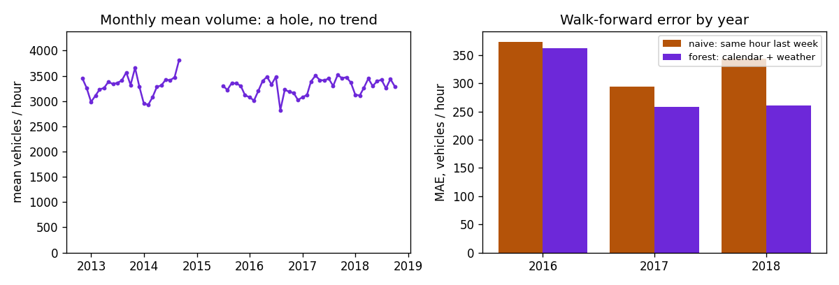

Monthly mean traffic volume over the six years, showing the ten-month hole and no trend, and the walk-forward error by year of the forest against the seasonal naive

Show the code for this figure

import matplotlib.pyplot as plt

fig, (a1, a2) = plt.subplots(1, 2, figsize=(10, 3.4))
monthly = d.set_index("t")["traffic_volume"].resample("M").mean()
a1.plot(monthly.index, monthly.values, marker="o", ms=2.5, color="#6d28d9")
a1.set_ylabel("mean vehicles / hour")
a1.set_title("Monthly mean volume: a hole, no trend")
a1.set_ylim(0, monthly.max() * 1.15)
x = np.arange(len(wf))
a2.bar(x - 0.2, wf["naive last-week MAE"], 0.4, label="naive: same hour last week", color="#b45309")
a2.bar(x + 0.2, wf["forest MAE"], 0.4, label="forest: calendar + weather", color="#6d28d9")
a2.set_xticks(x)
a2.set_xticklabels(wf.index)
a2.set_ylabel("MAE, vehicles / hour")
a2.set_title("Walk-forward error by year")
a2.legend(fontsize=8)
fig.tight_layout()
fig.savefig("metro-volume-and-walk-forward.png", dpi=120)
plt.show()

The forest beats the seasonal naive in each of the three years, by 3% in 2016, when it has the least training data, 13% in 2017 and 24% in 2018: the margin grows with the training window and shows no sign of decaying.

6. What to say

Hourly traffic on this road is a schedule: a table of mean volume by hour and weekday explains 94% of the variance a year ahead, “same hour last week” 89%, and a forest on the calendar 95%, with weather adding nothing. The forest’s error is below the seasonal naive’s in each of three walk-forward years, by 3% to 24%, with the margin growing as the training window grows. A shuffled split gives the same score as the chronological one because the mean volume has not changed in six years; that is a property of this series, not of shuffled splits. A quarter of the raw rows were duplicate timestamps and one in twenty hours is missing, so every lag was built against the actual clock rather than by row position.

Takeaways

Check the clock before the values. Duplicate timestamps, gaps and sentinels are three separate lines of code, and none of them appear in a summary table.
Build lags against timestamps, not row positions. A gap of ten months turns a row-based “yesterday” into last year.
A shuffled split lies when the level moves. Print the mean of the target by year. If it is flat, the shuffled score may be honest; if it is not, it is not. Either way, report the chronological one.
On a regular series the calendar is the lag. Adding last week’s value to a model that already knows the hour and the weekday adds little; the naive forecast is the baseline precisely because it is that calendar in one number.
Weather that adds nothing is worth reporting. Four columns removed is a simpler model, and the finding that they did not matter is part of the result.

Related: the load-forecasting study for lags relative to the horizon and walk-forward by month; common data-quality traps by dataset type; choosing a train/test split.