Attacking your own result

Once a signal scores on the hold-out, the next job is to try to make the result go away. Two attacks apply to every signal, and one or two sensitivity checks follow from whatever the interrogation found. The worked example throughout is the one-day reversal signal from the case study.

import pandas as pd, numpy as np

df = pd.read_csv("all_stocks_5yr.csv")
df["date"] = pd.to_datetime(df["date"])
df = df.rename(columns={"Name": "ticker"}).sort_values(["ticker", "date"]).reset_index(drop=True)
per = df.groupby("ticker").size()
df = df[df["ticker"].isin(per[per >= 1000].index)].copy()
g = df.groupby("ticker")
df["ret"] = g["close"].pct_change()
df["fwd_ret"] = g["ret"].shift(-1)
df["sig1"] = -df["ret"]
df = df.dropna(subset=["ret", "fwd_ret"])
cut, embargo = pd.Timestamp("2016-06-30"), pd.Timedelta(days=7)
test = df[df["date"] > cut + embargo].copy()

def daily_ic(d, sig, tgt="fwd_ret"):
    return d.groupby("date")[[sig, tgt]].apply(lambda x: x[sig].corr(x[tgt], method="spearman")).dropna()

def report(ic, label):
    m, s, n = ic.mean(), ic.std(), len(ic)
    print("%-26s mean IC %+.4f   t = %+.2f   hit = %.2f   days = %d" % (label, m, m / (s / np.sqrt(n)), (ic > 0).mean(), n))

ic = daily_ic(test, "sig1")
report(ic, "hold-out, all")

hold-out, all              mean IC +0.0156   t = +1.98   hit = 0.55   days = 399

Attack 1: is it stable?

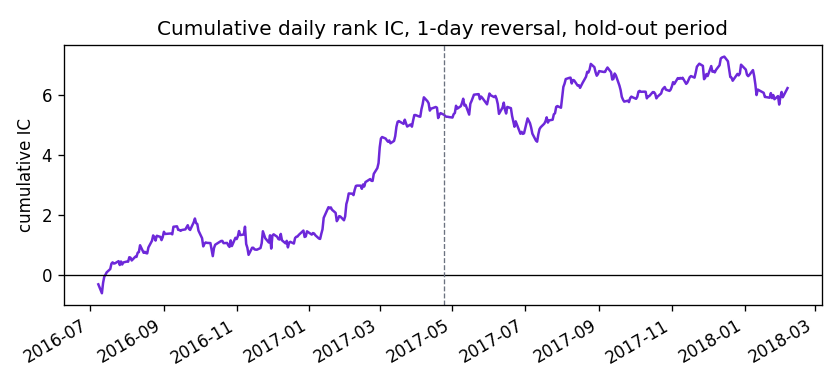
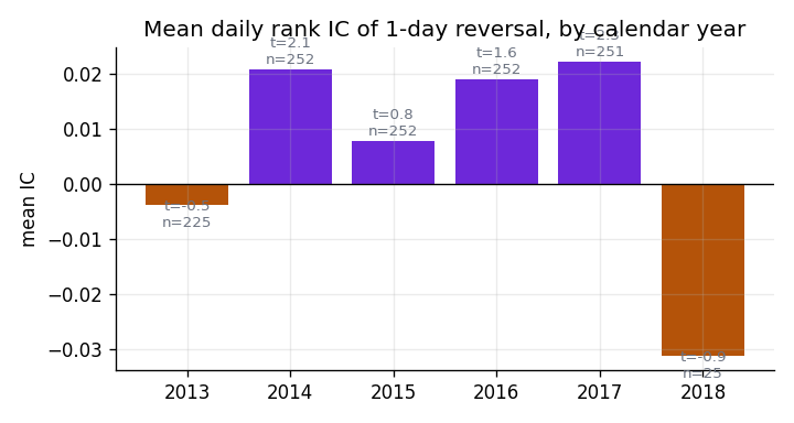
Three looks at the same question. Halves of the hold-out, the cumulative IC over time, and the IC by calendar year.

mid = test["date"].iloc[len(test) // 2]
report(ic[ic.index <= mid], "hold-out, 1st half")
report(ic[ic.index > mid], "hold-out, 2nd half")

hold-out, 1st half         mean IC +0.0267   t = +2.35   hit = 0.55   days = 200
hold-out, 2nd half         mean IC +0.0045   t = +0.41   hit = 0.55   days = 199

Almost all of the out-of-sample effect sits in the first half. Either it is decaying, or it is regime-dependent; either way the relationship is not stationary and the report has to say so. The cumulative IC plot shows the same thing as a picture: the line climbs and then goes flat.

ic_all = daily_ic(df, "sig1")                      # both periods, for the by-year view only
by_year = ic_all.groupby(ic_all.index.year).agg(["mean", "std", "count"])
by_year["t"] = by_year["mean"] / (by_year["std"] / np.sqrt(by_year["count"]))
print(by_year.round(4).to_string())

        mean     std  count       t
date                               
2013 -0.0039  0.1211    225 -0.4773
2014  0.0208  0.1565    252  2.1114
2015  0.0078  0.1500    252  0.8217
2016  0.0189  0.1832    252  1.6400
2017  0.0221  0.1532    251  2.2900
2018 -0.0312  0.1730     25 -0.9027

Positive in four of five full years, never large, and 2018 is twenty-five days of noise. Show this as a bar chart and say “positive in most years, not all”.

Attack 2: could anyone use it?

An IC says the ranking is informative. It says nothing about whether the information survives the cost of acting on it. Long the top decile of the signal, short the bottom, rebalance every day; then ask how much of the book turns over and what transaction cost would eat the gross return.

def long_short(d, sig):
    def one(x):
        q = pd.qcut(x[sig].rank(method="first"), 10, labels=False)
        return x.loc[q == 9, "fwd_ret"].mean() - x.loc[q == 0, "fwd_ret"].mean()
    return d.groupby("date")[[sig, "fwd_ret"]].apply(one).dropna()

def top_decile_turnover(d, sig):
    tops = d.groupby("date")[[sig, "ticker"]].apply(
        lambda x: set(x.loc[pd.qcut(x[sig].rank(method="first"), 10, labels=False) == 9, "ticker"]))
    changes = [1 - len(a & b) / max(len(a), 1) for a, b in zip(tops.values[:-1], tops.values[1:])]
    return float(np.mean(changes))

ls = long_short(test, "sig1")
gross = ls.mean() * 1e4                                   # bps per day
sharpe = ls.mean() / ls.std() * np.sqrt(252)
to = top_decile_turnover(test, "sig1")                    # share of the long book replaced each day
breakeven = gross / (2 * to)                              # two legs, each turning over `to` per day
print("gross %.2f bps/day   annualised Sharpe %.2f   top-decile turnover %.0f%%   break-even round-trip cost %.1f bps"
      % (gross, sharpe, 100 * to, breakeven))

gross 4.12 bps/day   annualised Sharpe 0.77   top-decile turnover 85%   break-even round-trip cost 2.4 bps

Gross, it looks fine. But 85% of the long book is replaced every day, so costs are paid on nearly the whole portfolio daily, and the edge is gone at a round-trip cost of about 2.4 basis points, which is what only the best-executed institutional flow pays. The honest summary is signal exists, edge does not clear costs. The cost sweep is the chart for it.

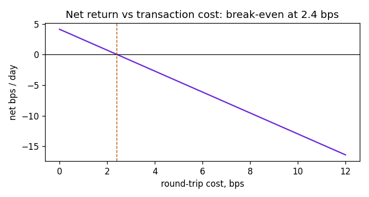
The break-even is a linear model: net = gross − 2 × turnover × cost. It ignores market impact and the fact that turnover could be reduced by holding longer, both of which are follow-ups, not corrections.

Sensitivity: the rows you were worried about

The interrogation found 46 rows with moves over 25%, some of them unadjusted corporate actions, and the decision was to keep them but use ranks. Check that the decision did not carry the result.

extreme = df.loc[df["ret"].abs() > 0.25, ["date", "ticker"]]
kept = test.merge(extreme.assign(_x=1), on=["date", "ticker"], how="left")
report(daily_ic(kept[kept["_x"].isna()], "sig1"), "hold-out, extremes out")

hold-out, extremes out     mean IC +0.0156   t = +1.97   hit = 0.55   days = 399

Unchanged to the third decimal, which is the point of ranks. Had the number moved, the finding would have been “the effect is in the extreme rows”, which is a different and more suspicious result.

The other standard sensitivity is by subgroup: large names against small, or sectors if the file has them. Split the tickers by median dollar volume into halves and score each.

dollar = (df["close"] * df["volume"]).groupby(df["ticker"]).median()
big = dollar[dollar >= dollar.median()].index
report(daily_ic(test[test["ticker"].isin(big)], "sig1"), "hold-out, larger half")
report(daily_ic(test[~test["ticker"].isin(big)], "sig1"), "hold-out, smaller half")

hold-out, larger half      mean IC +0.0139   t = +1.64   hit = 0.55   days = 399
hold-out, smaller half     mean IC +0.0182   t = +2.18   hit = 0.56   days = 399

Present in both halves, somewhat stronger in the less-traded names. That leans the same way as the cost story (thinner names, wider spreads, more bid-ask bounce) without proving it, and it is a fact the presentation should contain rather than hide.

What to say

One sentence per attack, in order: it is concentrated in the first half of the hold-out; it turns over 85% a day and dies at 2.4 bps; it survives dropping the extreme rows; it is a little stronger in the smaller names. A result that has been attacked this way and survived some of the attacks is worth more than one that was never attacked and looks cleaner.