
Repeated subjects: a model that learns who, not how ill
Voice recordings from 42 people, about 140 each, and a clinician's symptom score to predict. A random split gives an R² above 0.9; holding out whole subjects gives a negative one. What the model actually learned, and which question each split answers.
Most tables with an identifier column have more than one row per identifier: customers with many orders, stores with many weeks, machines with many readings, patients with many visits. Any model fitted on such a table can learn two different things, what distinguishes the entities from each other and what predicts the outcome within an entity, and a random train/test split cannot tell you which one it learned. This study shows the difference on a small public medical table, where the gap between the two is about as large as it gets.
The data: the Parkinson’s telemonitoring set from the UCI repository (parkinsons_updrs.csv): 5,875 voice recordings made at home by 42 people with early-stage Parkinson’s over about six months, sixteen numerical measures of each recording (jitter, shimmer, noise ratios and a few nonlinear summaries), the subject’s age and sex, the time since recruitment, and two clinician-assessed symptom scores. The one used here is total_UPDRS, where higher means worse.
The question, as it arrived: “Can the voice measures predict the UPDRS score?”
That sentence hides two questions. Given more recordings from a patient already in the trial, can we track their score? And given a recording from a patient we have never seen, can we estimate their score? They need different validation designs, they have different answers, and a random split answers neither.
1. Understand the data
import pandas as pd, numpy as np

df = pd.read_csv("parkinsons_updrs.csv").rename(columns={"subject#": "subject"})
voice = [c for c in df.columns if c not in ("subject", "age", "sex", "test_time", "motor_UPDRS", "total_UPDRS")]
print(df.shape, "| subjects:", df["subject"].nunique(), "| voice measures:", len(voice))
per = df.groupby("subject").size()
print("recordings per subject: min %d  median %d  max %d" % (per.min(), per.median(), per.max()))
span = df.groupby("subject")["test_time"].agg(lambda s: s.max() - s.min())
print("days covered per subject: median %.0f  (test_time runs %.1f -> %.1f)" % (span.median(), df["test_time"].min(), df["test_time"].max()))
print("exact duplicate rows:", df.duplicated().sum(), "| nulls:", int(df.isna().sum().sum()))
print(df["total_UPDRS"].describe().round(1).to_string())
(5875, 22) | subjects: 42 | voice measures: 16
recordings per subject: min 101 median 141 max 168
days covered per subject: median 171 (test_time runs -4.3 -> 215.5)
exact duplicate rows: 0 | nulls: 0
count 5875.0
mean 29.0
std 10.7
min 7.0
25% 21.4
50% 27.6
75% 36.4
max 55.0One row is one recording. Forty-two subjects, about 140 recordings each, spread over roughly half a year. No duplicates, no nulls, a target that runs from 7 to 55 with a standard deviation of about 11.
The single most important number for this table is how much of that variance sits between subjects rather than within them:
y = df["total_UPDRS"]
subj_mean = df.groupby("subject")["total_UPDRS"].transform("mean")
print("variance of total_UPDRS: %.1f | between-subject: %.1f | within-subject: %.1f" % (y.var(), subj_mean.var(), (y - subj_mean).var()))
print("share of variance that is 'which subject': %.2f" % (subj_mean.var() / y.var()))
print("distinct (age, sex) pairs among %d subjects: %d" % (df["subject"].nunique(), df[["age", "sex"]].drop_duplicates().shape[0]))
variance of total_UPDRS: 114.5 | between-subject: 106.9 | within-subject: 7.6
share of variance that is 'which subject': 0.93
distinct (age, sex) pairs among 42 subjects: 31Ninety-three percent of the variance in the target is explained by knowing which subject the row belongs to. Whatever else happens below, a model that can work out who a recording came from can reach an R² in the nineties without knowing anything about symptoms. And age and sex almost identify the subject on their own: 42 people, 31 distinct (age, sex) pairs.
One more thing from the documentation shipped with the data: the two scores were assessed by a clinician at a few clinic visits and linearly interpolated to the recording dates. Within a subject, the target is therefore a straight line between visits. That matters for what “tracking a known patient” can even mean.
2. The prediction boundary
The voice measures are computed from the recording being scored, so they are known when the prediction is made. Age, sex and time since recruitment are known. The clinician’s score is what we are predicting. There is no post-event column in this table; the leakage here is structural, not a stray column. See prediction boundaries.
3. Three validation designs
Each answers a different question. All three are run on the same rows with the same models so that only the split changes.
from sklearn.model_selection import KFold, GroupKFold

random_folds = list(KFold(5, shuffle=True, random_state=0).split(df))
grouped_folds = list(GroupKFold(5).split(df, groups=df["subject"]))
df["pos"] = df.groupby("subject")["test_time"].rank(pct=True)     # 0..1: position in the subject's own timeline
later = (df["pos"] > 0.7).values
within_folds = [(np.where(~later)[0], np.where(later)[0])]
designs = {"random rows": random_folds, "known subjects, later recordings": within_folds, "unseen subjects": grouped_folds}
for name, folds in designs.items():
    tr, te = folds[0]
    shared = len(set(df.iloc[tr]["subject"]) & set(df.iloc[te]["subject"]))
    print("%-34s first fold: %d train rows, %d test rows, %d subjects appear in both" % (name, len(tr), len(te), shared))
random rows first fold: 4700 train rows, 1175 test rows, 42 subjects appear in both
known subjects, later recordings first fold: 4112 train rows, 1763 test rows, 42 subjects appear in both
unseen subjects first fold: 4738 train rows, 1137 test rows, 0 subjects appear in both- Random rows. Five-fold, shuffled. Every subject is in both train and test of every fold. This is what
train_test_splitdoes by default and it answers no question anyone asked. - Known subjects, later recordings. For each subject, the first 70% of their recordings by time train, the last 30% test. Answers: can we track a patient we are already monitoring?
- Unseen subjects.
GroupKFoldon the subject id: each fold holds out eight or nine whole people. Answers: can we score a new patient?
4. Baselines
Each design gets the baseline that is honestly available to it. A model for a known patient may use that patient’s history; a model for an unseen patient may not.
def r2(y, yhat):
    return 1 - np.sum((y - yhat) ** 2) / np.sum((y - y.mean()) ** 2)

def cross_val(folds, predict_fn):
    """predict_fn(train_frame, test_frame) -> predictions for the test frame. Pooled out-of-fold R2 and MAE."""
    pred = np.full(len(df), np.nan)
    for tr, te in folds:
        pred[te] = predict_fn(df.iloc[tr], df.iloc[te])
    ok = ~np.isnan(pred)
    yy = df["total_UPDRS"].values[ok]
    return r2(yy, pred[ok]), np.mean(np.abs(yy - pred[ok]))

results = {}
def report(design, label, score):
    results[(design, label)] = score
    print("%-34s %-32s R2 %+.3f   MAE %.2f" % (design, label, score[0], score[1]))

global_mean = lambda tr, te: np.full(len(te), tr["total_UPDRS"].mean())
subject_mean = lambda tr, te: te["subject"].map(tr.groupby("subject")["total_UPDRS"].mean()).values
last_value = lambda tr, te: te["subject"].map(tr.sort_values("test_time").groupby("subject")["total_UPDRS"].last()).values
for design, folds in designs.items():
    report(design, "baseline: train mean", cross_val(folds, global_mean))
    if design != "unseen subjects":
        report(design, "baseline: subject's own mean", cross_val(folds, subject_mean))
    if design == "known subjects, later recordings":
        report(design, "baseline: subject's last score", cross_val(folds, last_value))
random rows baseline: train mean R2 -0.000 MAE 8.66
random rows baseline: subject's own mean R2 +0.932 MAE 2.13
known subjects, later recordings baseline: train mean R2 -0.018 MAE 8.65
known subjects, later recordings baseline: subject's own mean R2 +0.825 MAE 3.68
known subjects, later recordings baseline: subject's last score R2 +0.946 MAE 1.81
unseen subjects baseline: train mean R2 -0.020 MAE 8.79Two baselines that use nothing but the identifier column already reach an R² above 0.9. For a known patient, their last recorded score is a better prediction than anything below, which follows directly from the interpolated target: between clinic visits the score moves slowly along a line, so the most recent value is nearly right. Any model claiming to track known patients has to beat 0.95, not zero.
5. The same models under the three designs
A linear model on the sixteen voice measures, a random forest on the same, a forest with age and sex added, and a forest given only age and sex, which cannot possibly know anything about the voice.
from sklearn.linear_model import LinearRegression
from sklearn.ensemble import RandomForestRegressor

def fitted(model, feats):
    return lambda tr, te: model().fit(tr[feats].values, tr["total_UPDRS"].values).predict(te[feats].values)

rf = lambda: RandomForestRegressor(n_estimators=60, min_samples_leaf=2, random_state=0, n_jobs=-1)
models = [("linear, 16 voice measures", LinearRegression, voice),
          ("forest, 16 voice measures", rf, voice),
          ("forest, voice + age + sex", rf, voice + ["age", "sex"]),
          ("forest, age + sex only", rf, ["age", "sex"])]
for design, folds in designs.items():
    for label, model, feats in models:
        report(design, label, cross_val(folds, fitted(model, feats)))
random rows linear, 16 voice measures R2 +0.094 MAE 8.34
random rows forest, 16 voice measures R2 +0.375 MAE 6.53
random rows forest, voice + age + sex R2 +0.914 MAE 2.26
random rows forest, age + sex only R2 +0.844 MAE 3.24
known subjects, later recordings linear, 16 voice measures R2 +0.065 MAE 8.35
known subjects, later recordings forest, 16 voice measures R2 +0.292 MAE 7.16
known subjects, later recordings forest, voice + age + sex R2 +0.802 MAE 3.85
known subjects, later recordings forest, age + sex only R2 +0.705 MAE 4.79
unseen subjects linear, 16 voice measures R2 -0.084 MAE 9.22
unseen subjects forest, 16 voice measures R2 -0.192 MAE 9.53
unseen subjects forest, voice + age + sex R2 -0.573 MAE 10.93
unseen subjects forest, age + sex only R2 -0.544 MAE 10.50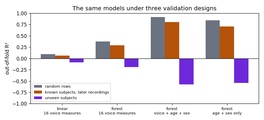
Show the code for this figure
import matplotlib.pyplot as plt

labels = [m[0] for m in models]
colours = ["#6b7280", "#b45309", "#6d28d9"]
fig, ax = plt.subplots(figsize=(7.5, 3.4))
w = 0.26
for i, design in enumerate(designs):
    vals = [results[(design, l)][0] for l in labels]
    ax.bar(np.arange(len(labels)) + (i - 1) * w, vals, w, label=design, color=colours[i])
ax.axhline(0, color="k", lw=0.8)
ax.set_xticks(range(len(labels)))
ax.set_xticklabels([l.replace(", ", "\n") for l in labels], fontsize=8)
ax.set_ylabel("out-of-fold R²")
ax.set_ylim(-1.0, 1.0)
ax.legend(fontsize=8, loc="lower left")
ax.set_title("The same models under three validation designs")
fig.tight_layout()
fig.savefig("parkinsons-r2-by-design.png", dpi=120)
plt.show()
Read the table by column.
Random rows. The forest with voice, age and sex scores an R² of 0.91. The forest given only age and sex, two columns that say nothing about the recording, scores 0.84. The forest given only voice is well below both, and the linear model is near 0.1. The pattern is the tell: a two-column model with no information about the voice gets most of the way to the full model, because the two columns nearly name the subject and the forest memorises each subject’s typical score. Neither beats the subject’s-own-mean baseline.
Known subjects, later recordings. Everything drops, and every model is beaten by the subject’s-last-score baseline. Voice measures add nothing to knowing the patient’s recent history.
Unseen subjects. Every forest has a negative R², meaning it does worse on new people than predicting the training mean. The forests that looked best under a random split are the worst here, because what they learned (which age-and-sex combination has which score) is a table of the 33 training subjects, applied to nine people who are not in it. The linear model on voice is roughly at zero.
6. What the model actually learned
Two direct checks. First, can the voice measures identify the person?
from sklearn.ensemble import RandomForestClassifier
acc = []
for tr, te in random_folds:
    clf = RandomForestClassifier(n_estimators=60, random_state=0, n_jobs=-1).fit(df.iloc[tr][voice].values, df.iloc[tr]["subject"].values)
    acc.append((clf.predict(df.iloc[te][voice].values) == df.iloc[te]["subject"].values).mean())
print("a forest asked to name the SUBJECT from the 16 voice measures alone: accuracy %.2f (chance %.3f)" % (np.mean(acc), 1 / df["subject"].nunique()))
a forest asked to name the SUBJECT from the 16 voice measures alone: accuracy 0.56 (chance 0.024)A voice is a fingerprint. The sixteen measures identify the speaker more than half the time out of 42, so under a random split the forest on voice alone is partly a subject classifier with a lookup table attached. That is the 0.3–0.4 it scores there, and it is why that number vanishes for new subjects.
Second, do the voice measures relate to the score across people, or within a person over time? Both correlations, side by side:
within = df[voice + ["total_UPDRS"]] - df.groupby("subject")[voice + ["total_UPDRS"]].transform("mean")
between = df.groupby("subject")[voice + ["total_UPDRS"]].mean()
corr = pd.DataFrame({"between subjects (42 means)": between.corr(method="spearman")["total_UPDRS"],
                     "within subject (demeaned rows)": within.corr(method="spearman")["total_UPDRS"]}).drop("total_UPDRS")
print(corr.round(3).sort_values("between subjects (42 means)").to_string())
between subjects (42 means) within subject (demeaned rows)
HNR -0.268 0.029
DFA -0.159 -0.015
Jitter(Abs) 0.182 0.001
Shimmer:APQ3 0.193 -0.018
Shimmer:DDA 0.193 -0.018
Shimmer:APQ5 0.204 -0.023
PPE 0.225 -0.009
Shimmer 0.231 -0.021
Shimmer(dB) 0.236 -0.021
Jitter:PPQ5 0.242 -0.008
Jitter(%) 0.243 -0.009
Jitter:RAP 0.262 -0.009
Jitter:DDP 0.262 -0.009
Shimmer:APQ11 0.264 -0.030
RPDE 0.265 0.001
NHR 0.328 -0.013Between subjects there is a modest relationship: people whose voices are on average noisier and more variable tend to have higher scores, with rank correlations of 0.2 to 0.3 on 42 points, which is weak evidence at that sample size. Within a subject the correlations are essentially zero: as one person’s score drifts over six months, their voice measures do not drift with it. That is the whole result. The information in this table about symptoms lives at the level of the person, and there are only 42 people.
7. What to say
Under a random split the voice measures plus age and sex predict the clinician’s score with an R² of about 0.9. That number is not about the voice: age and sex alone reach the same score, because they identify the subject and 93% of the target’s variance is which subject it is. For patients already being monitored, the last recorded score is a better predictor than any model. For patients not in the training data, no model here beats predicting the average, and the voice measures show no within-person relationship with the score over six months. With 42 subjects, the honest answer to “can voice predict the score for a new patient” is “not detectably in this data”.
Takeaways
- Count rows per entity before choosing a split. If the answer is “many”, a random split is measuring how well the model recognises entities, and
GroupKFold(or a hand-built entity hold-out) is the design that answers the question about new entities. - Decompose the target’s variance into between-entity and within-entity. When most of it is between, any feature correlated with identity (age, sex, location, an account number, a voice) will look predictive under a random split.
- Give each design its own baseline. For known entities the entity’s own history is the baseline, and it is often unbeatable; for unseen entities it is the training mean.
- A cheap model with no domain information that matches the expensive one is not a sign the problem is easy. It is a sign both are reading the same identifier.
- Between-entity and within-entity correlations are different questions. Check both before claiming a feature “predicts” the outcome.
The same design question appears wherever entities repeat: stores and weeks, machines and readings, customers and transactions, monitoring sites and hours. For a panel where the entity explains very little and time explains most, see twelve monitoring sites, one sky, which is the same three-way comparison with the opposite outcome. For the general rule, see choosing a train/test split.