
Predicting taxi tips: the column that contains the answer
A non-financial table with the two traps that matter most outside finance. A total column that includes the target, and a payment type for which the target was never recorded. What each does to a model, measured on a hold-out.
Not every table is a panel of prices. This study is the workflow applied to a small public table of taxi trips, chosen because it contains, in miniature, the two data problems that decide most non-financial modelling exercises: a column that is an arithmetic function of the target, and a category in which the target was never recorded.
The question, as it arrived: “Predict the tip.”
The data: the 6,433-row New York taxi sample distributed with seaborn (taxis.csv): one row per trip in March 2019 with pickup and dropoff times, passengers, distance, fare, tip, tolls, total, taxi colour, payment type and pickup/dropoff zones.
1. Interrogation
import pandas as pd, numpy as np

df = pd.read_csv("taxis.csv")
df["pickup"] = pd.to_datetime(df["pickup"])
df["dropoff"] = pd.to_datetime(df["dropoff"])
print(df.shape, "| pickup range:", df["pickup"].min(), "->", df["pickup"].max())
print("exact duplicate rows:", df.duplicated().sum(), "| nulls:", df.isna().sum()[lambda s: s > 0].to_dict())
dur = (df["dropoff"] - df["pickup"]).dt.total_seconds() / 60
print("duration (min): median %.1f  max %.1f | non-positive: %d | zero distance: %d | zero passengers: %d" % (dur.median(), dur.max(), (dur <= 0).sum(), (df["distance"] == 0).sum(), (df["passengers"] == 0).sum()))
print(df[["distance", "fare", "tip", "tolls", "total"]].describe().loc[["mean", "50%", "max"]].round(2).to_string())
(6433, 14) | pickup range: 2019-02-28 23:29:03 -> 2019-03-31 23:43:45
exact duplicate rows: 0 | nulls: {'payment': 44, 'pickup_zone': 26, 'dropoff_zone': 45, 'pickup_borough': 26, 'dropoff_borough': 45}
duration (min): median 10.9 max 107.7 | non-positive: 6 | zero distance: 51 | zero passengers: 96
distance fare tip tolls total
mean 3.02 13.09 1.98 0.33 18.52
50% 1.64 9.50 1.70 0.00 14.16
max 36.70 150.00 33.20 24.02 174.82One row is a trip. No duplicates, a month of data, a few impossible trips (zero minutes, zero distance, zero passengers) that are noted and kept since they do not affect the tip question.
Trap 1: total contains tip
resid = df["total"] - df["fare"] - df["tip"] - df["tolls"]
print("total - fare - tip - tolls, most common values:", resid.round(2).value_counts().head(4).to_dict())
print("corr(total, tip) = %.3f   corr(fare, tip) = %.3f" % (df["total"].corr(df["tip"]), df["fare"].corr(df["tip"])))
total - fare - tip - tolls, most common values: {3.3: 2625, 3.8: 1510, 4.3: 838, 0.8: 629}
corr(total, tip) = 0.646 corr(fare, tip) = 0.489The residual takes a handful of values: fixed surcharges. total is fare plus tip plus tolls plus a surcharge, so a model given total can recover the tip by subtraction. It is excluded from every feature set below, and one model is fitted with it to show what would have happened.
Trap 2: cash tips are not recorded
print(df.groupby("payment")["tip"].agg(["count", "mean", lambda s: (s == 0).mean()]).rename(columns={"<lambda_0>": "share_zero"}).round(3).to_string()) count mean share_zero
payment
cash 1812 0.000 1.000
credit card 4577 2.782 0.099Every one of 1,812 cash trips has a tip of exactly zero. Cash tips exist; the meter does not see them. Those rows are not examples of “no tip”; they are examples of “tip unknown”, and a model trained on them learns a fact about the recording system rather than about tipping. The study restricts to card payments and says so. See leaked columns and labels that aren’t labels.
2. The protocol
Target. tip in dollars, on credit-card trips only.
Features. fare, distance, tolls, passengers. Never total.
Split. By pickup time: build on trips before 2019-03-24, check on trips from 2019-03-24. (A month of data has no room for an embargo of any size; the target does not look forward, so none is needed.)
Score. Mean absolute error and R² on the check period.
Baselines. The build-period mean tip; the build-period median tip; and a fixed share of the fare, with the share fitted on the build period.
card = df[df["payment"] == "credit card"].sort_values("pickup")
cutd = pd.Timestamp("2019-03-24")
tr, te = card[card["pickup"] < cutd], card[card["pickup"] >= cutd]
print("build %d trips (%s -> %s) | check %d trips (%s -> %s)" % (len(tr), tr["pickup"].min().date(), tr["pickup"].max().date(), len(te), te["pickup"].min().date(), te["pickup"].max().date()))

def fit(cols):
    X = np.column_stack([np.ones(len(tr))] + [tr[c].values for c in cols])
    return np.linalg.lstsq(X, tr["tip"].values, rcond=None)[0]

def predict(beta, d, cols):
    return np.column_stack([np.ones(len(d))] + [d[c].values for c in cols]) @ beta

def score(yhat, label):
    y = te["tip"].values
    print("%-40s MAE %.3f   R2 %+.3f" % (label, np.mean(np.abs(y - yhat)), 1 - np.sum((y - yhat) ** 2) / np.sum((y - y.mean()) ** 2)))
build 3503 trips (2019-03-01 -> 2019-03-23) | check 1074 trips (2019-03-24 -> 2019-03-31)3. Baselines, then models
score(np.full(len(te), tr["tip"].mean()), "baseline: build mean")
score(np.full(len(te), tr["tip"].median()), "baseline: build median")
share = tr["tip"].sum() / tr["fare"].sum()
score(share * te["fare"].values, "baseline: %.3f x fare" % share)
for cols in (["fare"], ["fare", "distance"], ["fare", "distance", "tolls", "passengers"]):
    score(predict(fit(cols), te, cols), "OLS on " + " + ".join(cols))
baseline: build mean MAE 1.587 R2 -0.004
baseline: build median MAE 1.548 R2 -0.090
baseline: 0.199 x fare MAE 1.223 R2 +0.427
OLS on fare MAE 1.179 R2 +0.442
OLS on fare + distance MAE 1.180 R2 +0.443
OLS on fare + distance + tolls + passengers MAE 1.175 R2 +0.450The honest picture: a fixed 20% of the fare explains 43% of the variance in tips; a regression on the fare adds a little; distance, tolls and passengers add almost nothing beyond the fare. Tips are mostly a share of the fare plus noise, and that is the finding.
4. What the leaked column would have done
score(predict(fit(["total"]), te, ["total"]), "OLS on total  (LEAKED)")
beta = fit(["total", "fare", "tolls"])
score(predict(beta, te, ["total", "fare", "tolls"]), "OLS on total + fare + tolls  (LEAKED)")
print("coefficients (intercept, total, fare, tolls):", beta.round(3))
OLS on total (LEAKED) MAE 0.989 R2 +0.621
OLS on total + fare + tolls (LEAKED) MAE 0.498 R2 +0.913
coefficients (intercept, total, fare, tolls): [-2.065 0.695 -0.648 -0.63 ]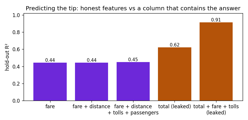
Show the code for this figure
import matplotlib.pyplot as plt

def holdout_r2(cols):
    y, yhat = te["tip"].values, predict(fit(cols), te, cols)
    return 1 - np.sum((y - yhat) ** 2) / np.sum((y - y.mean()) ** 2)

sets = [("fare", ["fare"]), ("fare + distance", ["fare", "distance"]),
        ("fare + distance\n+ tolls + passengers", ["fare", "distance", "tolls", "passengers"]),
        ("total (leaked)", ["total"]), ("total + fare + tolls\n(leaked)", ["total", "fare", "tolls"])]
vals = [holdout_r2(c) for _, c in sets]
fig, ax = plt.subplots(figsize=(7, 3.4))
ax.bar([s for s, _ in sets], vals, color=["#6d28d9"] * 3 + ["#b45309"] * 2)
for i, v in enumerate(vals):
    ax.text(i, v + 0.01, "%.2f" % v, ha="center", fontsize=9)
ax.set_ylabel("hold-out R²")
ax.set_ylim(0, 1.02)
ax.set_title("Predicting the tip: honest features vs a column that contains the answer")
fig.tight_layout()
fig.savefig("taxi-leak-r2.png", dpi=120)
plt.show()
With total, fare and tolls together the model reaches an R² of 0.91, and the coefficients show it has learned to subtract: roughly tip ≈ 0.7 × total − 0.65 × fare − 0.63 × tolls − 2, which is the identity from Trap 1 with the surcharge averaged into the intercept. It is not a model of tipping; it is a model of the meter’s arithmetic. Nobody could use it, because at prediction time the total is not known before the tip is.
5. What the unrecorded labels would have done
allp = df[df["payment"].isin(["credit card", "cash"])].sort_values("pickup")
tra = allp[allp["pickup"] < cutd]
tea = allp[allp["pickup"] >= cutd]
X = np.column_stack([np.ones(len(tra)), tra["fare"].values, tra["distance"].values])
beta_all = np.linalg.lstsq(X, tra["tip"].values, rcond=None)[0]
score(predict(beta_all, te, ["fare", "distance"]), "OLS fare + distance, trained incl. cash")
OLS fare + distance, trained incl. cash MAE 1.496 R2 +0.270The same two features, trained on all rows and scored on the card trips: R² falls from 0.44 to 0.27. The model has been taught that a large share of trips tip nothing and predicts too low everywhere. That is the cost of treating “not recorded” as “zero”.
6. What to say
Tips on card trips are about 20% of the fare plus noise; a one-feature regression on the fare explains 44% of the hold-out variance, and nothing else in the table adds materially to it. Two columns had to be handled before that could be measured: total, which contains the tip and would have produced an R² of 0.91 that means nothing, and cash trips, for which the tip is unrecorded and which would have pulled every prediction down.
What I would do with another day
- Time-of-day and day-of-week features, since tipping norms differ between the airport run and the 2 a.m. ride.
- Tip as a percentage of the fare as the target, which removes the fare from the answer and asks the more interesting question: who tips more than 20%?
- A random forest on the same chronological split, to check whether zone-to-zone interactions carry anything the linear model misses. Reported the same way, on the same hold-out.