Feature decay across horizons

A signal that works one day ahead may work for a week or die by day two. Scoring it against forward outcomes of increasing horizon answers two questions at once: how long the information lasts, and therefore how often a position based on it would have to be turned over.

Setup

import pandas as pd, numpy as np

df = pd.read_csv("all_stocks_5yr.csv")
df["date"] = pd.to_datetime(df["date"])
df = df.rename(columns={"Name": "ticker"}).sort_values(["ticker", "date"]).reset_index(drop=True)
per = df.groupby("ticker").size()
df = df[df["ticker"].isin(per[per >= 1000].index)].copy()
g = df.groupby("ticker")
df["ret"] = g["close"].pct_change()
df["sig1"] = -df["ret"]
df["vol20"] = g["ret"].transform(lambda x: x.rolling(20).std())
df["relvol"] = df["volume"] / g["volume"].transform(lambda x: x.rolling(20).mean())
test_start = pd.Timestamp("2016-06-30") + pd.Timedelta(days=7)

def daily_ic(d, sig, tgt):
    return d.groupby("date")[[sig, tgt]].apply(lambda x: x[sig].corr(x[tgt], method="spearman")).dropna()

def line(ic, h):
    m, s, n = ic.mean(), ic.std(), len(ic)
    t = m / (s / np.sqrt(n))
    return "h = %2d   mean IC %+.4f   naive t %+.2f   overlap-adjusted t %+.2f   days %d" % (h, m, t, t / np.sqrt(h), n)

Cumulative horizon: signal against the next h days’ return

for h in (1, 2, 3, 5, 10, 20):
    col = "fwd%d" % h
    df[col] = g["ret"].transform(lambda x: x.shift(-h).rolling(h).sum())     # days t+1 .. t+h
    d = df[df["date"] > test_start].dropna(subset=["sig1", col])
    print(line(daily_ic(d, "sig1", col), h))

h =  1   mean IC +0.0156   naive t +1.98   overlap-adjusted t +1.98   days 399
h =  2   mean IC +0.0091   naive t +1.19   overlap-adjusted t +0.84   days 398
h =  3   mean IC +0.0061   naive t +0.80   overlap-adjusted t +0.46   days 397
h =  5   mean IC +0.0031   naive t +0.42   overlap-adjusted t +0.19   days 395
h = 10   mean IC +0.0076   naive t +1.06   overlap-adjusted t +0.34   days 390
h = 20   mean IC +0.0031   naive t +0.43   overlap-adjusted t +0.10   days 380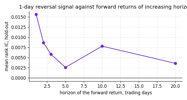

For horizons above one day, consecutive days’ targets overlap, so the naive t-statistic overstates the evidence; dividing by $\sqrt{h}$ is the conservative correction. See t-statistics from repeated looks.

Day-by-day: signal against the return on day t+k alone

The cumulative view can hide where the information sits. The day-by-day view shows it.

for k in (1, 2, 3, 4, 5):
    df["r_k"] = g["ret"].shift(-k)
    d = df[df["date"] > test_start].dropna(subset=["sig1", "r_k"])
    ic = daily_ic(d, "sig1", "r_k")
    print("day t+%d alone   mean IC %+.4f   t %+.2f   days %d" % (k, ic.mean(), ic.mean() / (ic.std() / np.sqrt(len(ic))), len(ic)))

day t+1 alone   mean IC +0.0156   t +1.98   days 399
day t+2 alone   mean IC -0.0036   t -0.49   days 398
day t+3 alone   mean IC -0.0057   t -0.82   days 397
day t+4 alone   mean IC -0.0045   t -0.66   days 396
day t+5 alone   mean IC +0.0085   t +1.21   days 395

For one-day reversal the information is entirely in the next day and there is nothing on days two to five. A position would have to be turned over daily, which is what the cost analysis finds.

A signal with a slower decay: size instead of sign

Relative volume predicts the size of tomorrow’s move. Sizes are persistent, so the same exercise gives a different shape.

df = df.replace([np.inf, -np.inf], np.nan)
for h in (1, 2, 3, 5, 10, 20):
    col = "size%d" % h
    df[col] = g["ret"].shift(-h).abs() / df["vol20"]                        # the move on day t+h alone, normalised
    d = df[df["date"] > test_start].dropna(subset=["relvol", col])
    ic = daily_ic(d, "relvol", col)
    print("day t+%2d alone   mean IC %+.4f   t %+.2f   days %d" % (h, ic.mean(), ic.mean() / (ic.std() / np.sqrt(len(ic))), len(ic)))

day t+ 1 alone   mean IC +0.1010   t +29.36   days 399
day t+ 2 alone   mean IC +0.0632   t +20.62   days 398
day t+ 3 alone   mean IC +0.0495   t +15.08   days 397
day t+ 5 alone   mean IC +0.0305   t +9.61   days 395
day t+10 alone   mean IC +0.0226   t +7.10   days 390
day t+20 alone   mean IC +0.0204   t +6.50   days 380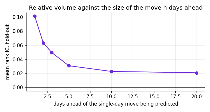

The IC halves by day two and is still clearly positive at day twenty. Volatility information is slow; direction information, on this data, does not survive the night. See the relative volume case study.

Reading a decay curve

• Falls to zero after day one: the effect is short-lived, possibly microstructure (bid-ask bounce). High turnover is unavoidable.
• Decays smoothly over weeks: a persistent state variable. Positions can be held; costs matter less.
• Rises with horizon: suspicious. Either the target’s overlap is inflating things or the signal is proxying for a slow-moving characteristic, and the overlap-adjusted t is the number to trust.