
Does today's market return predict tomorrow's?
The single-series version of the reversal question, under a fixed protocol. The protocol's score finds nothing; a measure the protocol did not name finds something consistent. What to do with a result like that.
The reversal study read “is tomorrow’s return predictable?” cross-sectionally. This study takes the other reading: does the market’s return today say anything about the market’s return tomorrow? It is a short study whose pre-registered score found nothing, and whose secondary measure found something consistent. Both halves of that sentence have to be reported, in that order, with the second labelled for what it is.
1. The question as I read it
- Single-series. One number per day: the equal-weight mean return across the stocks in the file.
- Horizon. One day.
- Score. The lag-1 autocorrelation, equivalently the OLS slope of tomorrow’s return on today’s. With its standard error.
- Repeats. There is no cross-section, so the repeats are calendar years and quarters, and the by-block numbers are the real evidence. See single series or panel.
- Baselines. Zero for the slope; for the sign, the share of up days (the majority-class rate).
2. The series
import pandas as pd, numpy as np

df = pd.read_csv("all_stocks_5yr.csv")
df["date"] = pd.to_datetime(df["date"])
df = df.rename(columns={"Name": "ticker"}).sort_values(["ticker", "date"]).reset_index(drop=True)
per = df.groupby("ticker").size()
df = df[df["ticker"].isin(per[per >= 1000].index)].copy()
df["ret"] = df.groupby("ticker")["close"].pct_change()

mkt = df.groupby("date")["ret"].mean().dropna()
m = pd.DataFrame({"r": mkt})
m["r_next"] = m["r"].shift(-1)
m = m.dropna()
print("days: %d | mean daily %.5f  std %.4f  min %.3f  max %.3f" % (len(m), m["r"].mean(), m["r"].std(), m["r"].min(), m["r"].max()))
days: 1257 | mean daily 0.00055 std 0.0080 min -0.041 max 0.032Equal-weight rather than cap-weighted because the file has no market caps; the survivorship bias of the file inflates the mean return but has little to do with day-to-day autocorrelation.
3. The protocol
Target. Tomorrow’s equal-weight market return. Signal. Today’s equal-weight market return. Split. Build to 2016-06-30; check from 2016-07-08; one-week embargo. Score. OLS slope of target on signal with its t-statistic; the same computed per year and per quarter as the repeats. Baselines. Slope of zero; for the sign, always predicting the majority class.
def ols(x, y):
    X = np.column_stack([np.ones(len(x)), x])
    beta, *_ = np.linalg.lstsq(X, y, rcond=None)
    resid = y - X @ beta
    se = np.sqrt(resid @ resid / (len(y) - 2) * np.linalg.inv(X.T @ X)[1, 1])
    return beta[1], se, beta[1] / se

cut, embargo = pd.Timestamp("2016-06-30"), pd.Timedelta(days=7)
for name, d in (("all", m), ("build", m[m.index <= cut]), ("check", m[m.index > cut + embargo])):
    slope, se, t = ols(d["r"].values, d["r_next"].values)
    print("%-6s slope %+.4f   se %.4f   t %+.2f   Spearman %+.4f   n %d" % (name, slope, se, t, d["r"].corr(d["r_next"], method="spearman"), len(d)))
all slope -0.0036 se 0.0282 t -0.13 Spearman -0.0680 n 1257
build slope +0.0110 se 0.0343 t +0.32 Spearman -0.0492 n 854
check slope -0.0707 se 0.0495 t -1.43 Spearman -0.1262 n 399Nothing in the slope on the build period; a negative slope on the check period with a t of −1.4, which would be reported as “nothing” even if it had been the only number.
The Spearman column, which was not the protocol’s score but is printed alongside it, disagrees. The rank correlation is −0.07 over all days and −0.13 on the check period, and with a naive standard error of about those are 2.4 and 2.5 standard errors from zero. A result that appears in the rank measure and not in the slope is the fat-tails signature in reverse: the largest market days are not following the pattern that the ordinary days follow. It has to be reported, and it has to face the same test as the slope, which is the per-block view.
4. The repeats: years and quarters
by_year = m.groupby(m.index.year).apply(lambda d: d["r"].corr(d["r_next"]))
by_year_sp = m.groupby(m.index.year).apply(lambda d: d["r"].corr(d["r_next"], method="spearman"))
print("per year, Pearson: ", by_year.round(3).to_dict())
print("per year, Spearman:", by_year_sp.round(3).to_dict())
for label, s in (("Pearson", by_year), ("Spearman", by_year_sp)):
    print("%-8s mean across years %+.4f   t %+.2f   n = %d   share < 0: %.2f" % (label, s.mean(), s.mean() / (s.std() / np.sqrt(len(s))), len(s), (s < 0).mean()))
by_q = m.groupby(m.index.to_period("Q")).apply(lambda d: d["r"].corr(d["r_next"], method="spearman") if len(d) > 10 else np.nan).dropna()
print("per quarter, Spearman: mean %+.4f   t %+.2f   n = %d   share < 0: %.2f" % (by_q.mean(), by_q.mean() / (by_q.std() / np.sqrt(len(by_q))), len(by_q), (by_q < 0).mean()))
per year, Pearson: {2013: -0.055, 2014: 0.015, 2015: 0.054, 2016: -0.051, 2017: -0.087, 2018: 0.124}
per year, Spearman: {2013: -0.071, 2014: -0.032, 2015: -0.043, 2016: -0.115, 2017: -0.111, 2018: -0.1}
Pearson mean across years +0.0001 t +0.00 n = 6 share < 0: 0.50
Spearman mean across years -0.0787 t -5.43 n = 6 share < 0: 1.00
per quarter, Spearman: mean -0.0832 t -3.04 n = 21 share < 0: 0.76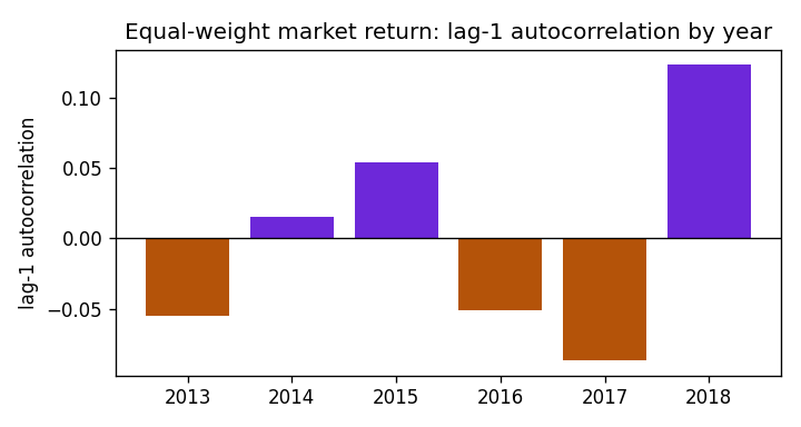
Show the code for this figure
import matplotlib.pyplot as plt

fig, ax = plt.subplots(figsize=(6, 3.2))
ax.bar(by_year.index.astype(str), by_year.values, color=["#6d28d9" if v > 0 else "#b45309" for v in by_year.values])
ax.axhline(0, color="k", lw=0.8)
ax.set_ylabel("lag-1 autocorrelation")
ax.set_title("Equal-weight market return: lag-1 autocorrelation by year")
fig.tight_layout()
fig.savefig("market-autocorr-by-year.png", dpi=120)
plt.show()
The Pearson sign flips from year to year and its mean across years is zero: the protocol’s score finds nothing, and the chart shows why. The Spearman version is negative in every one of the six years, in 76% of the quarters, and its mean across years is more than five standard errors from zero. In ranks, a relatively good day for the market is followed by a relatively poor one, consistently, and the effect is invisible to the slope because the largest days do not follow it.
This is a finding, and it is a post-hoc finding. The protocol named the slope as the score; the rank correlation was printed alongside it out of habit and turned out to disagree. The correct handling is not to pretend the protocol said Spearman all along, and not to bury the number either. It is to report the pre-registered result first, then the secondary result labelled as secondary, with the by-block evidence that makes it worth a follow-up, and to say that confirming it needs a protocol that names the rank measure in advance and a fresh period to test it on.
5. The sign, against the majority class
up = m["r_next"] > 0
same = (m["r"] > 0) == up
print("share of up days %.3f | 'same sign as today' %.3f | 'opposite sign' %.3f" % (up.mean(), same.mean(), (~same).mean()))
for lag in (1, 2, 3, 5, 10):
    print("lag %2d autocorrelation %+.4f" % (lag, m["r"].autocorr(lag)))
share of up days 0.558 | 'same sign as today' 0.472 | 'opposite sign' 0.528
lag 1 autocorrelation -0.0030
lag 2 autocorrelation -0.0256
lag 3 autocorrelation -0.0053
lag 5 autocorrelation -0.0349
lag 10 autocorrelation -0.0000Always saying “up” scores 55.8%. Neither sign rule beats it, including the “opposite sign” rule that the rank result would suggest: whatever the rank reversal is, it is not strong enough to call the direction of tomorrow better than the base rate. The longer Pearson lags are as close to zero as the first.
6. What to say
Under the protocol, there is no detectable one-day autocorrelation in the market’s return: the slope is zero on the build period, mildly negative and insignificant on the check period, and its per-year sign flips four times in six years. A rank correlation computed alongside, which the protocol did not name, is negative in every year and in three quarters out of four, with a t across years of −5. That is a consistent mild reversal in ranks that the slope cannot see, presumably because the largest market days go the other way. It is reported as a secondary, post-hoc observation; it does not improve on the majority-class rule for predicting the sign; and confirming it would need a protocol that names the rank measure in advance and a period this study has not looked at.
Two lessons. The first is the contrast with the cross-sectional reading: the same file and the same question in ordinary language, and one reading gives ~500 independent looks a day while the other gives one. When a question can be read cross-sectionally, read it that way first. The second is what a protocol is for. It did not stop the secondary result from being seen; it stopped it from being presented as the result.
What I would do with another day
- Re-run with the rank correlation as the pre-registered score, on data after 2018, since this file cannot provide an unlooked-at period any more.
- Ask why the slope and the ranks disagree: condition on the size of today’s move and check whether the very largest market days continue rather than reverse.
- Cap-weight the index if market caps can be found, since the equal-weight series over-represents small names, whose reversal is stronger.