
Flight delays: what is known two hours before departure
328,521 departures from three airports in one year, 21% of them more than fifteen minutes late. A model built from the schedule alone scores an AUC of 0.67; one that also uses the airport's observed delay state two hours before departure, 0.73. The weather at the departure hour, which nobody has in advance, adds nothing beyond the weather two hours earlier. How the moment of prediction decides the feature set, and how to encode four thousand aircraft without fooling yourself.
“Will this flight be delayed?” is not one question. Asked the day before, it can use the schedule. Asked two hours before departure, it can use the weather outside and the delays already piling up at the gate. Asked as the aircraft pushes back, it is not a prediction. This study builds the same classifier at each of those moments and measures what each moment is worth, then deals with the two things every flight table has: a rare-ish positive class and a few columns with thousands of levels.
The data: every flight that left the three New York airports in 2013 (nyc_flights.csv, from the nycflights13 collection, originally the US Bureau of Transportation Statistics on-time database), and hourly weather at each airport (nyc_weather.csv, from the same collection).
The question, as it arrived: “Predict which departures will be delayed.”
1. Understand the data
import pandas as pd, numpy as np

f = pd.read_csv("nyc_flights.csv")
f["sched"] = pd.to_datetime(f["time_hour"]).dt.tz_localize(None)     # scheduled departure, to the hour; the file stores it in UTC
cancelled = f["dep_time"].isna()
print(f.shape, "| flights with no departure time (cancelled): %d (%.2f%%)" % (cancelled.sum(), 100 * cancelled.mean()))
d = f[~cancelled].copy()
d["delayed"] = (d["dep_delay"] > 15).astype(int)
print("departures: %d | delayed by more than 15 minutes: %.3f | dep_delay median %.0f, 90th percentile %.0f, max %.0f minutes"
      % (len(d), d["delayed"].mean(), d["dep_delay"].median(), d["dep_delay"].quantile(0.9), d["dep_delay"].max()))
print("delay rate by scheduled hour:", d.groupby("hour")["delayed"].mean().round(2).to_dict())
print("delay rate by month:", d.groupby("month")["delayed"].mean().round(2).to_dict())
print("distinct values: carrier %d, origin %d, dest %d, tailnum %d, flight number %d" % (d["carrier"].nunique(), d["origin"].nunique(), d["dest"].nunique(), d["tailnum"].nunique(), d["flight"].nunique()))
(336776, 20) | flights with no departure time (cancelled): 8255 (2.45%)
departures: 328521 | delayed by more than 15 minutes: 0.215 | dep_delay median -2, 90th percentile 49, max 1301 minutes
delay rate by scheduled hour: {5: 0.06, 6: 0.07, 7: 0.08, 8: 0.11, 9: 0.12, 10: 0.14, 11: 0.16, 12: 0.18, 13: 0.22, 14: 0.23, 15: 0.27, 16: 0.29, 17: 0.3, 18: 0.31, 19: 0.35, 20: 0.36, 21: 0.37, 22: 0.32, 23: 0.26}
delay rate by month: {1: 0.19, 2: 0.2, 3: 0.22, 4: 0.23, 5: 0.23, 6: 0.29, 7: 0.3, 8: 0.22, 9: 0.14, 10: 0.15, 11: 0.15, 12: 0.28}
distinct values: carrier 16, origin 3, dest 104, tailnum 4037, flight number 3838One row is one scheduled departure. Two decisions before anything else. Cancelled flights (2.5%) have no delay; they are excluded here, and the result is a model of delay given that the flight goes, which should be said. The target is the industry’s convention, more than fifteen minutes late, which makes it a binary target with a 21% positive rate: not rare enough to break accuracy entirely, but enough that the majority-class rate is 79% before any model exists.
Two structures are visible already. The delay rate climbs all day, from 7% at 6 am to 37% at 9 pm, as delays propagate. And it moves by month, with a summer peak and an autumn trough, which matters for the split. The categorical columns run from 3 levels (origin) to 4,037 (aircraft tail number).
2. The prediction boundary, three times
| Known the day before | Known two hours before | Known only at departure |
|---|---|---|
| scheduled hour, weekday, carrier, origin, destination, distance, aircraft | the above, plus the weather observed at the origin two hours earlier, plus how late the flights scheduled two hours earlier actually left | the weather at the departure hour; the delay itself |
The middle column needs care. At two hours before a flight, every flight scheduled two hours earlier has either departed, in which case its delay is known, or is still waiting, in which case its delay is at least 120 minutes so far. Clipping observed delays at 120 makes the airport’s mean delay an honest feature: it uses exactly what a dispatcher could see. See prediction boundaries.
w = pd.read_csv("nyc_weather.csv")
w["time"] = pd.to_datetime(w["time_hour"]).dt.tz_localize(None)
wx = ["temp", "dewp", "humid", "wind_speed", "precip", "pressure", "visib"]
wk = w.drop_duplicates(["origin", "time"]).set_index(["origin", "time"])[wx]
wk.loc[wk["wind_speed"] > 100, "wind_speed"] = np.nan                     # one reading of over a thousand mph

def weather_before(hours, suffix):
    key = pd.MultiIndex.from_arrays([d["origin"], d["sched"] - pd.Timedelta(hours=hours)])
    block = wk.reindex(key)
    block.index = d.index
    return block.add_suffix(suffix)

d = pd.concat([d, weather_before(2, "_2h"), weather_before(0, "_now")], axis=1)
d["observed_delay"] = d["dep_delay"].clip(upper=120)                       # what is visible two hours later: departed, or waiting 120+ minutes
state = d.groupby(["origin", "sched"])["observed_delay"].mean()
key = pd.MultiIndex.from_arrays([d["origin"], d["sched"] - pd.Timedelta(hours=2)])
d["origin_state_2h"] = state.reindex(key).values
d["dow"] = d["sched"].dt.dayofweek
print("weather matched two hours before departure: %.3f of flights | origin state available: %.3f" % (d["temp_2h"].notna().mean(), d["origin_state_2h"].notna().mean()))
print("delay rate by decile of the origin's mean observed delay two hours earlier:")
print(d.groupby(pd.qcut(d["origin_state_2h"], 10, duplicates="drop"))["delayed"].mean().round(2).to_string())
weather matched two hours before departure: 0.996 of flights | origin state available: 0.913
delay rate by decile of the origin's mean observed delay two hours earlier:
origin_state_2h
(-18.001, -3.333] 0.09
(-3.333, -1.526] 0.10
(-1.526, 0.25] 0.13
(0.25, 2.269] 0.14
(2.269, 4.526] 0.16
(4.526, 7.133] 0.19
(7.133, 10.4] 0.22
(10.4, 15.125] 0.27
(15.125, 25.48] 0.37
(25.48, 120.0] 0.62The airport’s state two hours earlier sorts departures from a 9% delay rate to a 62% one. It is the strongest single feature in the table, and it is a lag feature on a time series that happens to be indexed by airport rather than by ticker.
3. Split and baselines
Train on January to August, test on September to December. The test months are not in the training data, so month cannot be a feature: a model given it would be asked about levels it has never seen. That also means the seasonal fall in delays across the test period is something the model has to live with, not something it can learn.
from sklearn.linear_model import LogisticRegression
from sklearn.metrics import roc_auc_score, average_precision_score, log_loss

tr, te = d[d["month"] <= 8], d[d["month"] >= 9]
y = te["delayed"].values
print("train: January-August, %d departures, delayed %.3f | test: September-December, %d departures, delayed %.3f" % (len(tr), tr["delayed"].mean(), len(te), y.mean()))
print("baseline: the constant training rate -> log-loss %.3f | majority-class accuracy %.3f" % (log_loss(y, np.full(len(y), tr["delayed"].mean())), 1 - y.mean()))

categorical = ["carrier", "origin", "dest", "hour"]

def design(frame, num, cat, columns=None):
    parts = [frame[num].astype(float)] if num else []
    if cat:
        parts.append(pd.get_dummies(frame[cat].astype(str), dtype=float))
    X = pd.concat(parts, axis=1)
    return X if columns is None else X.reindex(columns=columns, fill_value=0.0)

def evaluate(tr, te, num, cat, label):
    Xtr = design(tr, num, cat)
    Xte = design(te, num, cat, Xtr.columns)
    med = Xtr.median()                                                  # imputation learned on the training rows
    Xtr, Xte = Xtr.fillna(med), Xte.fillna(med)
    mu, sd = Xtr.mean(), Xtr.std().replace(0, 1)
    m = LogisticRegression(max_iter=3000).fit(((Xtr - mu) / sd).values, tr["delayed"].values)
    p = m.predict_proba(((Xte - mu) / sd).values)[:, 1]
    yy = te["delayed"].values
    print("%-60s AUC %.3f  PR-AUC %.3f  log-loss %.3f | mean p %.3f, actual %.3f" % (label, roc_auc_score(yy, p), average_precision_score(yy, p), log_loss(yy, p), p.mean(), yy.mean()))
    return p

wx_2h = [c + "_2h" for c in wx]
wx_now = [c + "_now" for c in wx]
print("--- known the day before: the schedule")
evaluate(tr, te, [], ["hour"], "scheduled hour only")
p_day = evaluate(tr, te, ["dow", "distance"], categorical, "hour + weekday + distance + carrier + origin + destination")
evaluate(tr, te, ["dow"], ["carrier", "hour"], "hour + weekday + carrier only")
print("--- known two hours before departure")
evaluate(tr, te, ["dow", "distance"] + wx_2h, categorical, "+ weather observed two hours earlier")
p_2h = evaluate(tr, te, ["dow", "distance"] + wx_2h + ["origin_state_2h"], categorical, "+ the origin's observed delay state two hours earlier")
print("--- not knowable in advance (an upper bound, not a model)")
evaluate(tr, te, ["dow", "distance"] + wx_now + ["origin_state_2h"], categorical, "weather at the departure hour instead of two hours earlier")
train: January-August, 218601 departures, delayed 0.235 | test: September-December, 109920 departures, delayed 0.177
baseline: the constant training rate -> log-loss 0.477 | majority-class accuracy 0.823
--- known the day before: the schedule
scheduled hour only AUC 0.648 PR-AUC 0.254 log-loss 0.458 | mean p 0.234, actual 0.177
hour + weekday + distance + carrier + origin + destination AUC 0.670 PR-AUC 0.283 log-loss 0.453 | mean p 0.235, actual 0.177
hour + weekday + carrier only AUC 0.670 PR-AUC 0.283 log-loss 0.453 | mean p 0.235, actual 0.177
--- known two hours before departure
+ weather observed two hours earlier AUC 0.703 PR-AUC 0.365 log-loss 0.435 | mean p 0.220, actual 0.177
+ the origin's observed delay state two hours earlier AUC 0.733 PR-AUC 0.451 log-loss 0.408 | mean p 0.197, actual 0.177
--- not knowable in advance (an upper bound, not a model)
weather at the departure hour instead of two hours earlier AUC 0.734 PR-AUC 0.451 log-loss 0.407 | mean p 0.197, actual 0.177Read down the AUC column. The scheduled hour alone is 0.65. The full schedule (route, carrier, distance) is 0.67, and carrier plus hour gets all of that: the 104 destinations and the distance add nothing once the carrier and the hour are known, a null result that saves a hundred dummy columns. Weather two hours out adds three points. The airport’s delay state adds three more, to 0.73. And the weather at the departure hour, which a real system would not have, is no better than the weather two hours earlier. The boundary cost nothing here; the honest feature set is as good as the impossible one.
The mean predicted probability is above the actual rate in every row: the model learned a 23% world and is being tested in a 18% one. That is the seasonal drift, and it is dealt with below.
4. Four thousand aircraft
The tail number identifies the aircraft. One-hot encoding it would add 4,037 columns; the tempting alternative is to replace each tail number by its delay rate. Done on the training rows and scored on the training rows, that looks like a real feature. Done honestly, it is not much of one.
gm = tr["delayed"].mean()
stats = tr.groupby("tailnum")["delayed"].agg(["mean", "size"])
shrunk = (stats["mean"] * stats["size"] + gm * 20) / (stats["size"] + 20)          # small counts pulled toward the base rate
print("aircraft in the test period never seen in training: %.3f" % (~te["tailnum"].isin(stats.index)).mean())
print("tailnum delay rate, fitted and scored on the same rows (training):    AUC %.3f" % roc_auc_score(tr["delayed"].values, tr["tailnum"].map(stats["mean"]).fillna(gm).values))
print("tailnum delay rate, fitted on training, scored on September-December: AUC %.3f" % roc_auc_score(y, te["tailnum"].map(shrunk).fillna(gm).values))
aircraft in the test period never seen in training: 0.010
tailnum delay rate, fitted and scored on the same rows (training): AUC 0.635
tailnum delay rate, fitted on training, scored on September-December: AUC 0.566In-sample the encoding scores 0.64, because each aircraft’s rate was computed from the very rows it is being scored on, including the row itself; an aircraft with three flights and one delay gets a rate of 0.33 that partly is its label. Out of time it scores 0.57, weak but real, and one aircraft in a hundred is new. Any target encoding must be fitted on rows the model is not scored on, either out-of-fold within training or, as here, on an earlier period, and shrunk toward the base rate for rare levels. See portable pandas idioms for the one-hot form with unseen levels.
5. Calibration, and the split that would have hidden the drift
dec = pd.qcut(p_2h, 10, labels=False, duplicates="drop")
print(pd.DataFrame({"p": p_2h, "y": y}).groupby(dec).agg(mean_predicted=("p", "mean"), delay_rate=("y", "mean")).round(3).T.to_string())
rng = np.random.RandomState(0)
idx = rng.permutation(len(d))
n = int(0.7 * len(d))
tr_r, te_r = d.iloc[idx[:n]], d.iloc[idx[n:]]
evaluate(tr_r, te_r, ["dow", "distance", "month"] + wx_2h + ["origin_state_2h"], categorical, "random 70/30 split, same features plus month")
0 1 2 3 4 5 6 7 8 9
mean_predicted 0.049 0.075 0.098 0.121 0.145 0.172 0.205 0.248 0.316 0.546
delay_rate 0.056 0.070 0.084 0.096 0.124 0.151 0.174 0.198 0.268 0.551
random 70/30 split, same features plus month AUC 0.754 PR-AUC 0.517 log-loss 0.440 | mean p 0.215, actual 0.215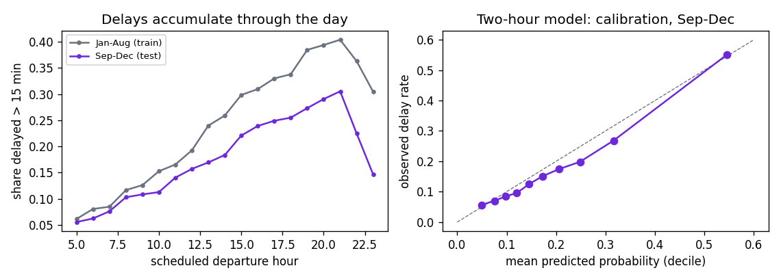
Show the code for this figure
import matplotlib.pyplot as plt

fig, (a1, a2) = plt.subplots(1, 2, figsize=(9.5, 3.4))
by_hour_tr = tr.groupby("hour")["delayed"].mean()
by_hour_te = te.groupby("hour")["delayed"].mean()
a1.plot(by_hour_tr.index, by_hour_tr.values, marker="o", ms=3, color="#6b7280", label="Jan-Aug (train)")
a1.plot(by_hour_te.index, by_hour_te.values, marker="o", ms=3, color="#6d28d9", label="Sep-Dec (test)")
a1.set_xlabel("scheduled departure hour")
a1.set_ylabel("share delayed > 15 min")
a1.set_title("Delays accumulate through the day")
a1.legend(fontsize=8)
cal = pd.DataFrame({"p": p_2h, "y": y}).groupby(dec).agg(mp=("p", "mean"), rate=("y", "mean"))
a2.plot([0, 0.6], [0, 0.6], ls="--", lw=0.8, color="#6b7280")
a2.plot(cal["mp"], cal["rate"], marker="o", color="#6d28d9")
a2.set_xlabel("mean predicted probability (decile)")
a2.set_ylabel("observed delay rate")
a2.set_title("Two-hour model: calibration, Sep-Dec")
fig.tight_layout()
fig.savefig("flights-hour-and-calibration.png", dpi=120)
plt.show()
Every decile over-predicts by a few points, except the top one, which is right: the ranking survives the season, the level does not. A model used in October would need its base rate re-anchored, which is a one-parameter fix, and would need it again in December when delays climb back. A random split with month as a feature reports 0.75 instead of 0.73 and a perfectly matched mean probability, and would have hidden both facts.
6. What to say
Whether a flight leaves more than fifteen minutes late can be predicted from the schedule alone with an AUC of 0.67, almost all of it from the hour of day and the carrier. Two hours before departure the airport’s own observed delays lift that to 0.73, and the weather observed at that point adds a little; the weather at the actual departure hour would add nothing more. Trained on January to August and tested on September to December, the model ranks well but over-predicts the delay rate, by two points with the full feature set and six with the schedule alone, because autumn is quieter, so the base rate needs re-anchoring by season. The aircraft identity carries a small amount of information when encoded honestly and a misleading amount when encoded on the same rows it is scored on.
Takeaways
- Write the prediction moment into the question, then sort every column into before, at, or after. The feature set follows; so does the number.
- Lag features exist outside forecasting. “How late are the flights that were due to leave two hours ago” is the same idea as “yesterday’s load”, and it needs the same care about what was observable.
- The impossible feature is a useful control. If the weather at departure had beaten the weather two hours earlier, the gap would measure what a forecast is worth. Here it measured nothing.
- Test on months the model has not seen, and expect the level to drift before the ranking does. Calibration by decile is the check.
- Target-encode out of sample or not at all. The in-sample version scores well for the same reason the random split on repeated subjects does.
- A hundred dummy columns that add nothing are a null result worth keeping: the honest model is smaller and easier to explain.
Related: hotel cancellations, where the post-booking columns are subtler and the threshold is worked through; bank marketing, where the positive class is rarer and the drift is larger; classification metrics.