Short-term reversal in daily equity returns

This is the research workflow run end to end on one question and one public file. Every number was produced by the code on this page.

The question, as it arrived: “Here are five years of daily prices for about five hundred US stocks. Is there anything predictable about tomorrow’s return?”

The data: all_stocks_5yr.csv from the plotly/datasets repository: S&P 500 constituents, daily OHLCV, 2013-02-08 to 2018-02-07, 619,040 rows, 505 tickers.

1. The question as I read it

Cross-sectional, not market-level. “Which stocks do better than others tomorrow?” rather than “does the market go up tomorrow?” Five hundred stocks a day is a lot of evidence; one market series is not. See single series or panel.
Horizon: one trading day. The question said “tomorrow”.
What counts as predictable: a signal computable today whose rank across stocks correlates with the rank of tomorrow’s return. That correlation, one per day, is the rank IC. Ranks, so that one extreme return cannot dominate a day.
Baseline: zero. If the IC is not reliably above zero, there is nothing.
First thing to test: the simplest idea. Do yesterday’s losers bounce and yesterday’s winners fade? Short-term reversal is a well-known effect, which makes it a good first baseline: if the pipeline cannot find it, the pipeline is broken.

2. The data, and three things wrong with it

import pandas as pd, numpy as np

df = pd.read_csv("all_stocks_5yr.csv")
df["date"] = pd.to_datetime(df["date"])
df = df.rename(columns={"Name": "ticker"}).sort_values(["ticker", "date"]).reset_index(drop=True)

print(df["date"].min().date(), "->", df["date"].max().date(), "|", df["date"].nunique(), "trading days |", df["ticker"].nunique(), "tickers")
print("nulls:", df.isna().sum()[lambda s: s > 0].to_dict(), "| duplicate (date, ticker):", df.duplicated(["date", "ticker"]).sum())
per = df.groupby("ticker").size()
print("rows per ticker: min", per.min(), " median", per.median(), " max", per.max(), "| tickers with < 1000 rows:", (per < 1000).sum())
df["ret"] = df.groupby("ticker")["close"].pct_change()
print("daily return: mean %.5f  std %.4f  min %.3f  max %.3f | rows with |return| > 25%%: %d" % (df["ret"].mean(), df["ret"].std(), df["ret"].min(), df["ret"].max(), (df["ret"].abs() > 0.25).sum()))

2013-02-08 -> 2018-02-07 | 1259 trading days | 505 tickers
nulls: {'open': 11, 'high': 8, 'low': 8} | duplicate (date, ticker): 0
rows per ticker: min 44  median 1259.0  max 1259 | tickers with < 1000 rows: 22
daily return: mean 0.00054  std 0.0161  min -0.626  max 1.010 | rows with |return| > 25%: 46

The three findings, each with a decision:

Twenty-two tickers have short histories: spin-offs and recent listings. They add noise at the edges and nothing else. → Dropped (under 1000 rows).
This is the index as it stood at the end of the period. Every company that left the index or went bust between 2013 and 2018 is missing. That is survivorship bias, and it flatters any “buy the losers” result, because the losers that kept losing are not in the file. → Cannot be fixed. Named on every result.
Forty-six rows with a move over 25%. A +101% day is a real event or an unadjusted corporate action, and there is no time to check forty-six. → Kept, neutralised by ranks. Two were checked by eye: one is a bad print that reverses the next day, one is a spin-off.

The null opens and highs are irrelevant to a study that uses only the close. Noted, moved on.

df = df[df["ticker"].isin(per[per >= 1000].index)].dropna(subset=["close"]).copy()
g = df.groupby("ticker")
df["ret"] = g["close"].pct_change()
df["fwd_ret"] = g["ret"].shift(-1)          # TARGET: tomorrow's return. shift(-1) looks forward.
df = df.dropna(subset=["ret", "fwd_ret"])
print(df["ticker"].nunique(), "tickers,", len(df), "rows")

483 tickers, 606376 rows

3. The protocol, fixed before any result

Protocol

Target. Tomorrow’s close-to-close return, per ticker. Signal. Minus today’s close-to-close return (losers rank high). Split. Everything to 2016-06-30 is where I may look and choose. Everything from 2016-07-08 is hold-out, reported once at the end. One-week embargo between them. Score. Mean daily cross-sectional Spearman IC, with its t-statistic across days and the share of days with IC > 0. Baseline. IC = 0. Rule. Anything I try is chosen on the build period and reported on both. I count how many things I try.

cut, embargo = pd.Timestamp("2016-06-30"), pd.Timedelta(days=7)
train = df[df["date"] <= cut].copy()
test = df[df["date"] > cut + embargo].copy()
print("build", train["date"].min().date(), "->", train["date"].max().date(), len(train), "| check", test["date"].min().date(), "->", test["date"].max().date(), len(test))

def daily_ic(d, sig, tgt="fwd_ret"):
    """One Spearman correlation per day, across all stocks that day."""
    return d.groupby("date")[[sig, tgt]].apply(lambda x: x[sig].corr(x[tgt], method="spearman")).dropna()

def report(ic, label):
    m, s, n = ic.mean(), ic.std(), len(ic)
    print("%-26s mean IC %+.4f   t = %+.2f   hit = %.2f   days = %d" % (label, m, m / (s / np.sqrt(n)), (ic > 0).mean(), n))

build 2013-02-11 -> 2016-06-30 411727 | check 2016-07-08 -> 2018-02-06 192717

4. Baseline: one-day reversal

train["sig1"] = -train["ret"]
test["sig1"] = -test["ret"]
ic_tr1 = daily_ic(train, "sig1")
ic_te1 = daily_ic(test, "sig1")
report(ic_tr1, "1-day reversal, build")
report(ic_te1, "1-day reversal, check")

1-day reversal, build      mean IC +0.0114   t = +2.18   hit = 0.53   days = 854
1-day reversal, check      mean IC +0.0156   t = +1.98   hit = 0.55   days = 399

Read out loud: the daily rank IC of one-day reversal is about 0.015 out of sample, t just under 2, positive on 55% of days. A small, real-looking reversal effect: small in that an IC of 0.015 is tiny per day, real-looking in that it is consistent across two independent periods.

That is a result, and from here there is something to present. Everything that follows is improvement that can be measured.

5. One hypothesis round

Idea, mechanism first: maybe reversal over five days is stronger than over one. A week of losses bounces harder than a day. Chosen on the build period, reported on both.

for d in (train, test):
    d["sig5"] = -d.groupby("ticker")["ret"].transform(lambda x: x.rolling(5).sum())
report(daily_ic(train.dropna(subset=["sig5"]), "sig5"), "5-day reversal, build")
report(daily_ic(test.dropna(subset=["sig5"]), "sig5"), "5-day reversal, check")

5-day reversal, build      mean IC +0.0152   t = +2.88   hit = 0.53   days = 850
5-day reversal, check      mean IC +0.0081   t = +1.04   hit = 0.51   days = 395

This is the most important block on the page. On the build period the five-day version looked better (t = 2.9 against 2.2). With only one period, it is the one anyone would have picked and presented. On the hold-out it is worse than the one-day version and not distinguishable from zero. That is what selection bias looks like from the inside: it never feels like cheating, it feels like picking the better one.

The honest report: I tried two things. The simpler one held up; the one that looked better in-sample didn’t.

6. Attack the result

Is it stable?

mid = test["date"].iloc[len(test) // 2]
report(ic_te1[ic_te1.index <= mid], "check, 1st half")
report(ic_te1[ic_te1.index > mid], "check, 2nd half")

check, 1st half            mean IC +0.0267   t = +2.35   hit = 0.55   days = 200
check, 2nd half            mean IC +0.0045   t = +0.41   hit = 0.55   days = 199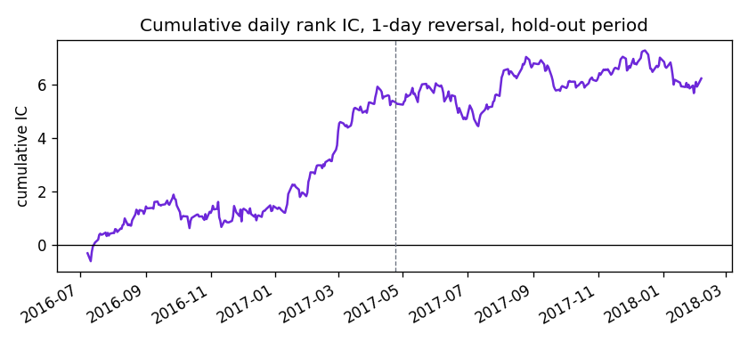

Cumulative daily rank IC of one-day reversal over the hold-out, with the midpoint marked

Show the code for this figure

import matplotlib.pyplot as plt

fig, ax = plt.subplots(figsize=(7, 3.2))
ic_te1.cumsum().plot(ax=ax, color="#6d28d9")
ax.axhline(0, color="k", lw=0.8)
ax.axvline(mid, color="#6b7280", ls="--", lw=0.8)
ax.set_title("Cumulative daily rank IC, 1-day reversal, hold-out period")
ax.set_ylabel("cumulative IC")
ax.set_xlabel("")
fig.tight_layout()
fig.savefig("reversal-cum-ic.png", dpi=120)
plt.show()

Almost all of the out-of-sample effect is in the first half of the hold-out (mid-2016 to spring 2017). In the second half it is essentially gone. Either it is decaying, which is well documented for short-term reversal as more capital trades it, or it is regime-dependent. Either way the relationship is not stationary and the report says so.

Could you use it?

Long the top decile of the signal, short the bottom, rebalanced daily.

def long_short(d, sig):
    def one(x):
        q = pd.qcut(x[sig].rank(method="first"), 10, labels=False)
        return x.loc[q == 9, "fwd_ret"].mean() - x.loc[q == 0, "fwd_ret"].mean()
    return d.groupby("date")[[sig, "fwd_ret"]].apply(one).dropna()

def top_decile_turnover(d, sig):
    tops = d.groupby("date")[[sig, "ticker"]].apply(
        lambda x: set(x.loc[pd.qcut(x[sig].rank(method="first"), 10, labels=False) == 9, "ticker"]))
    changes = [1 - len(a & b) / max(len(a), 1) for a, b in zip(tops.values[:-1], tops.values[1:])]
    return float(np.mean(changes))

ls = long_short(test, "sig1")
gross = ls.mean() * 1e4                                  # bps per day
to = top_decile_turnover(test, "sig1")                   # share of the long book replaced each day
print("long/short decile, gross: %.2f bps/day   annualised Sharpe %.2f" % (gross, ls.mean() / ls.std() * np.sqrt(252)))
print("top-decile turnover: %.0f%% per day" % (100 * to))
print("break-even round-trip cost ~ %.1f bps" % (gross / (2 * to)))

long/short decile, gross: 4.12 bps/day   annualised Sharpe 0.77
top-decile turnover: 85% per day
break-even round-trip cost ~ 2.4 bps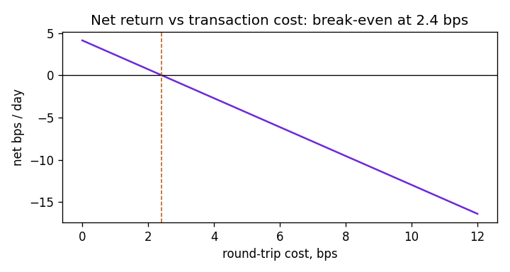

Net return per day against round-trip transaction cost, crossing zero at about 2.4 bps

Show the code for this figure

import matplotlib.pyplot as plt

costs = np.arange(0, 12.1, 0.5)
net = gross - 2 * to * costs
be = gross / (2 * to)
fig, ax = plt.subplots(figsize=(6, 3.2))
ax.plot(costs, net, color="#6d28d9")
ax.axhline(0, color="k", lw=0.8)
ax.axvline(be, color="#b45309", ls="--", lw=0.9)
ax.set_xlabel("round-trip cost, bps")
ax.set_ylabel("net bps / day")
ax.set_title("Net return vs transaction cost: break-even at %.1f bps" % be)
fig.tight_layout()
fig.savefig("reversal-cost-sweep.png", dpi=120)
plt.show()

Gross, it looks fine: 4 bps a day, Sharpe 0.8. But the signal changes almost completely every day. 85% of the long book is replaced daily, so costs are paid on nearly the whole portfolio, every day. It survives only below about 2.4 bps round-trip, which is roughly what the best-executed institutional flow pays and well below what anyone else does.

Signal exists; edge does not clear costs.

Sensitivity

Does the decision to keep the 46 extreme rows carry the result?

extreme = df.loc[df["ret"].abs() > 0.25, ["date", "ticker"]]
kept = test.merge(extreme.assign(_x=1), on=["date", "ticker"], how="left")
report(daily_ic(kept[kept["_x"].isna()], "sig1"), "check, extremes removed")

check, extremes removed    mean IC +0.0156   t = +1.97   hit = 0.55   days = 399

Unchanged, which is what ranks are for.

7. What I would do with another day

Ranked, and the first one already done because it was cheap:

Rule out bid-ask bounce. Closing prices alternate between bid and ask, which mechanically produces one-day reversal. Test: skip a day between signal and target.
Test for decay properly. A rolling IC by year rather than two halves.
Condition on volume. Does reversal after a high-volume day differ from reversal after a quiet one?

for d in (train, test):
    d["sig1_skip"] = -d.groupby("ticker")["ret"].shift(1)        # yesterday's return, so the target is two days after the signal's day
report(daily_ic(train.dropna(subset=["sig1_skip"]), "sig1_skip"), "skip-a-day, build")
report(daily_ic(test.dropna(subset=["sig1_skip"]), "sig1_skip"), "skip-a-day, check")

skip-a-day, build          mean IC +0.0073   t = +1.59   hit = 0.52   days = 853
skip-a-day, check          mean IC -0.0036   t = -0.49   hit = 0.49   days = 398

With one day skipped the effect is gone on the hold-out. That is consistent with a large part of the one-day reversal being microstructure rather than a slow-moving mispricing, and it belongs in the report as a caveat on the result, not as a footnote. The horizon decay page shows the same thing day by day.

The presentation

Seven slides, one sentence and one number or chart each:

#	Title	The sentence
1	The question as I read it	Cross-sectional, one day ahead, rank IC against a zero baseline.
2	The data, and three things wrong with it	483 tickers over 2013–18; survivorship-biased; 22 short histories dropped; extremes kept but ranked.
3	How I decided what counts	Time split at June 2016, one-week embargo, hold-out reported once. Fixed before any result.
4	Baseline: one-day reversal	Out of sample: IC +0.016, t ≈ 2, positive on 55% of days. Small and real-looking.
5	What else I tried	Five-day reversal beat it in-sample and lost out of sample. I tried two things; the simpler one held.
6	Does it hold, and can you use it	Concentrated in the first half of the hold-out; 85% daily turnover; dies at ~2.4 bps round-trip.
7	What I’d do with another day	Skip-a-day test (done: effect vanishes); rolling IC by year; condition on volume.

The questions, answered from this page

Why rank correlation? Forty-six rows have moves over 25%; a raw correlation would let one of them decide the day. On the hold-out the Pearson version gives +0.006 (t 0.8) against Spearman’s +0.016 (t 2.0).
Is 0.015 significant? t ≈ 2 over 399 days, having tried two things rather than two hundred. Borderline yes; I would want more data before believing the size of it.
Isn’t this just bid-ask bounce? Partly, at least. Skipping a day removes the hold-out effect.
Why did the five-day version fail? It didn’t fail; it looked better in one period and worse in the next, which is what noise does with two candidates. That is why the hold-out was fixed first.
Would you trade it? Not at this turnover. The edge has to beat about 2.4 bps round-trip, which it does not for anyone but the best-executed desks. Slow it down, hold longer, trade less, then re-test.
What about survivorship? The file has only the survivors, so the losers that kept losing are missing and the reversal is flattered. It cannot be fixed with this file; it would need the point-in-time constituent list.